Builds on NumPy arrays and matrices and provides lots of functions that perform scientific calculations on them.
See, for example, these submodules:
Integration (scipy.integrate): Provides functions for numerical integration, including single and multiple integrals, as well as solving ordinary differential equations (ODEs).
Optimization (scipy.optimize): Offers optimization algorithms for finding the minimum or maximum of a function, both constrained and unconstrained, and for curve fitting.
Interpolation (scipy.interpolate): Contains functions for interpolating data, including linear, polynomial, and spline interpolation.
Linear Algebra (scipy.linalg): Provides functions for performing linear algebra operations, such as solving linear systems, computing eigenvalues and eigenvectors, and singular value decomposition (SVD).
Statistics (scipy.stats): Contains a wide range of probability distributions and statistical functions for calculating statistics, generating random numbers, and performing hypothesis testing.
Signal Processing (scipy.signal): Offers functions for signal processing, including filtering, spectral analysis, and waveform generation.
Fast Fourier Transform (scipy.fft): Provides functions for computing the discrete Fourier transform (DFT) and its inverse, as well as for working with Fourier transforms in general.
Sparse matrices (scipy.sparse): Contains functions for working with sparse matrices, including creating sparse matrices, performing matrix-vector multiplication, and solving linear systems.
Spatial algorithms (scipy.spatial): Provides functions for working with spatial data structures and algorithms, such as nearest-neighbor queries and Delaunay triangulations.
Image Processing (scipy.ndimage): Offers functions for image processing tasks, such as filtering, morphological operations, and measurements on images.
Example: integration
\[
y = \int_{0}^{1}(x^2 + 2x) dx
\]
import scipy.integrate as spi# Define the function to be integrateddef f(x):return x**2+2*x# Calculate the definite integral of f(x) from 0 to 1result, error = spi.quad(f, 0, 1)print("Result:", result)print("Error:", error)
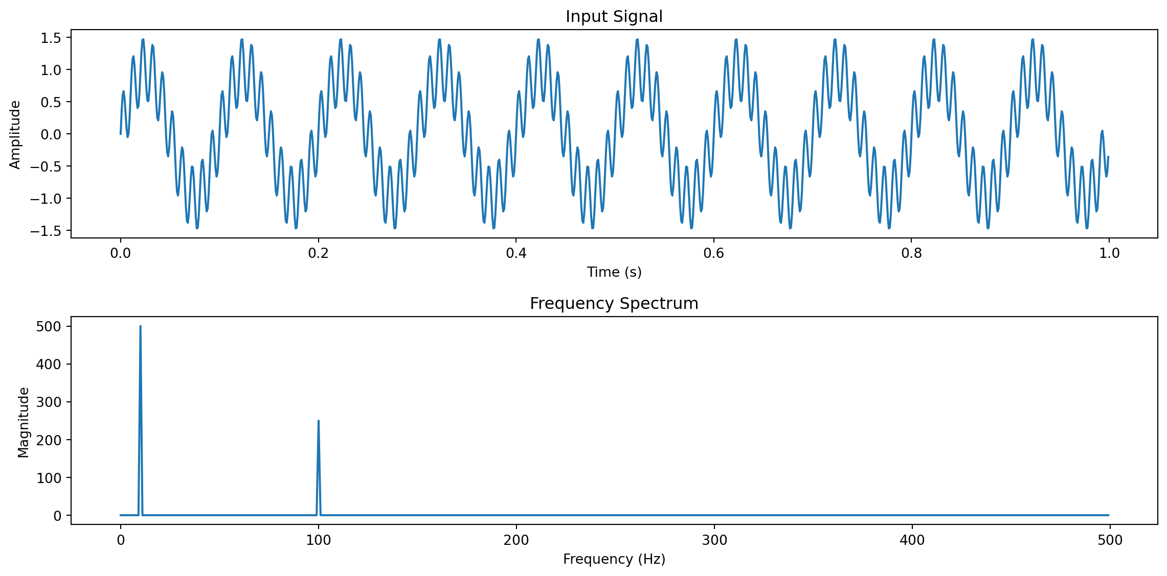
Example: calculating the frequency spectrum of a signal
import numpy as npimport matplotlib.pyplot as pltfrom scipy.fft import fft, fftfreq# Generate a sample signalfs =1000# Sampling frequencyt = np.linspace(0, 1, fs, endpoint=False) # Time vector from 0 to 1 secondf1, f2 =10, 100# Frequencies of the two components of the signalsignal = np.sin(2* np.pi * f1 * t) +0.5* np.sin(2* np.pi * f2 * t) # Signal with two components# Compute the FFTfft_result = fft(signal)magnitude = np.abs(fft_result)frequencies = fftfreq(len(signal), 1/fs)# Plot the signalplt.figure(figsize=(12, 6))plt.subplot(2, 1, 1)plt.plot(t, signal)plt.title('Input Signal')plt.xlabel('Time (s)')plt.ylabel('Amplitude')# Plot the frequency spectrumplt.subplot(2, 1, 2)plt.plot(frequencies[:fs//2], magnitude[:fs//2]) # Plot only the positive frequenciesplt.title('Frequency Spectrum')plt.xlabel('Frequency (Hz)')plt.ylabel('Magnitude')plt.tight_layout()plt.show()
Exercise: plotting a Voronoi diagram from a random collection of points.