NumPy Basics

• NumPy aims to provide an array object that is up to 50x faster than traditional Python lists. It is called ndarray.
• They also can be multidimensional and have a lot of supporting mathematical operations.

For example, observe some differences:

import numpy as np

list1 = [15.5, 25.11, 19.0]
list2 = [12.2, 1.3, 6.38] 

# Create two 1-dimensional (1D) arrays
# with the elements of the above lists
array1 = np.array(list1)
array2 = np.array(list2)

# Concatenate two lists
print('Concatenation of list1 and list2 =', end=' ')
print(list1 + list2)
print()

# Sum two lists
print('Sum of list1 and list2 =', end=' ')
for i in range(len(list1)):
    print(list1[i] + list2[i], end=' ')  
print('\n')

# Sum two 1D arrays
print('Sum of array1 and array2 =', end=' ')
print(array1 + array2)

Concatenation of list1 and list2 = [15.5, 25.11, 19.0, 12.2, 1.3, 6.38]

Sum of list1 and list2 = 27.7 26.41 25.38 

Sum of array1 and array2 = [27.7  26.41 25.38]

Some array properties

1. Shape: The shape of an array is a tuple of integers indicating the size of the array along each dimension. For a 1D array, the shape is (n,), for a 2D array, it’s (m, n), and so on.

import numpy as np

arr = np.array([[1, 2, 3], [4, 5, 6]])
print(arr.shape)

(2, 3)

2. Size: The total number of elements in the array is given by the size attribute.

import numpy as np

arr = np.array([[1, 2, 3], [4, 5, 6]])
print(arr.size)

6

3. Data Type (dtype): NumPy arrays are homogeneous, meaning all elements must have the same data type. The dtype attribute specifies the data type of the array elements.

import numpy as np

arr = np.array([1, 2, 3])
print(arr.dtype)

int64

4. Dimension (ndim): The number of dimensions of an array is given by the ndim attribute.

import numpy as np

arr = np.array([1, 2, 3])
print(arr.ndim)  # Output: 1

1

Array creation

In NumPy, there are several ways to create arrays. Here are some common methods:

1. np.array(): Convert a Python list or tuple to an array.

import numpy as np

arr = np.array([1, 2, 3, 4, 5])

2. np.arange(): Create an array with evenly spaced values within a given interval.

import numpy as np

arr = np.arange(0, 10, 2)  # Array from 0 to 10 with step size 2

3. np.linspace(): Create an array with evenly spaced values over a specified interval.

import numpy as np

arr = np.linspace(0, 1, 5)  # Array with 5 values from 0 to 1

4. np.zeros(): Create an array filled with zeros.

import numpy as np

arr = np.zeros((3, 3))  # 3x3 array of zeros

5. np.eye(): Create a 2D array with ones on the diagonal and zeros elsewhere (identity matrix).

import numpy as np

arr = np.eye(3)  # 3x3 identity matrix

These are just a few examples. The library provides many more functions and options for creating arrays with specific properties.

Array indexing and slicing

• Indexing is quite similar to indexing in Python lists. You can access individual elements of an array using square brackets [].
• The big difference: for multi-dimensional arrays, you can use a comma-separated tuple of indices.
  • This also works for slicing!

import numpy as np

# 1D array
arr1d = np.array([1, 2, 3, 4, 5])
print(arr1d[0])  # Output: 1

# 2D array
arr2d = np.array([[1, 2, 3], [4, 5, 6], [7, 8, 9]])
print(arr2d[0, 0])  # Output: 1
print(arr2d[0:2, 1:3])  # Output: [[2, 3], [5, 6]]

• Another nice feature is boolean indexing. You can use boolean arrays to index elements based on a condition.

import numpy as np

arr = np.array([1, 2, 3, 4, 5])
print(arr > 3)
print(arr[arr > 3])

[False False False  True  True]
[4 5]

Array manipulation

import numpy as np

# Reshape
arr = np.arange(1, 10)
reshaped_arr = arr.reshape(3, 3)
print(reshaped_arr)

# Concatenate
arr1 = np.array([[1, 2], [3, 4]])
arr2 = np.array([[5, 6], [7, 8]])
concatenated_arr = np.concatenate((arr1, arr2), axis=1)
print(concatenated_arr)

# Split
arr = np.arange(1, 10)
split_arr = np.split(arr, 3)
print(split_arr)

[[1 2 3]
 [4 5 6]
 [7 8 9]]
[[1 2 5 6]
 [3 4 7 8]]
[array([1, 2, 3]), array([4, 5, 6]), array([7, 8, 9])]

Some applications

Statistical aggregations

import numpy as np

arr = np.array([[1, 2], [3, 4]])

# Mean
print(np.mean(arr))

# Sum
print(np.sum(arr))

# Minimum
print(np.min(arr))

# Maximum
print(np.max(arr))

2.5
10
1
4

Statistical distributions

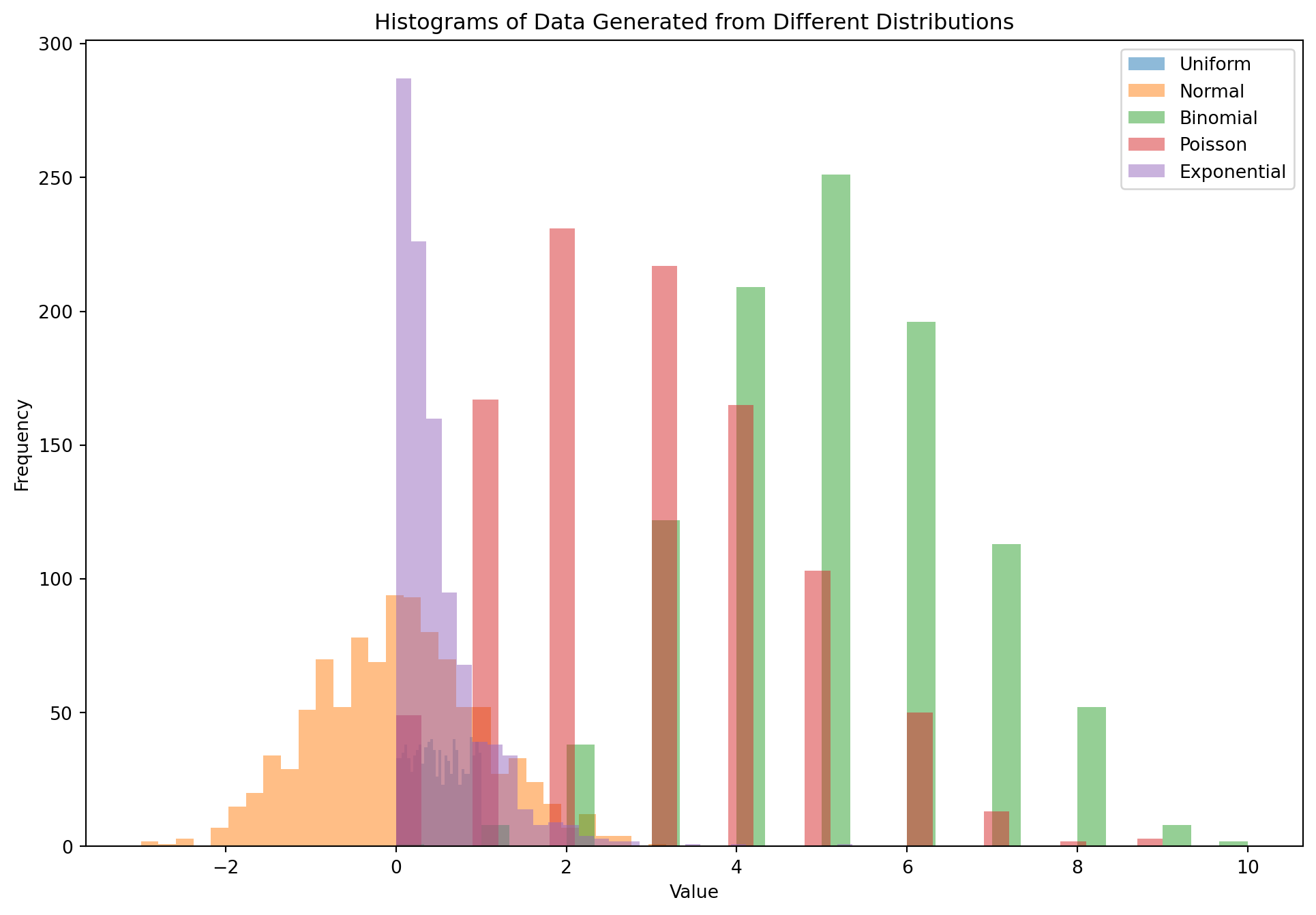
import numpy as np
import matplotlib.pyplot as plt

# Set seed for reproducibility
np.random.seed(0)

# Generate data from different distributions
data_uniform = np.random.uniform(0, 1, 1000)
data_normal = np.random.normal(0, 1, 1000)
data_binomial = np.random.binomial(10, 0.5, 1000)
data_poisson = np.random.poisson(3, 1000)
data_exponential = np.random.exponential(0.5, 1000)

# Plot histograms of the generated data
plt.figure(figsize=(12, 8))
plt.hist(data_uniform, bins=30, alpha=0.5, label='Uniform')
plt.hist(data_normal, bins=30, alpha=0.5, label='Normal')
plt.hist(data_binomial, bins=30, alpha=0.5, label='Binomial')
plt.hist(data_poisson, bins=30, alpha=0.5, label='Poisson')
plt.hist(data_exponential, bins=30, alpha=0.5, label='Exponential')
plt.legend()
plt.title('Histograms of Data Generated from Different Distributions')
plt.xlabel('Value')
plt.ylabel('Frequency')
plt.show()

Linear algebra

import numpy as np

# Matrix multiplication
arr1 = np.array([[1, 2], [3, 4]])
arr2 = np.array([[5, 6], [7, 8]])
print(np.matmul(arr1, arr2))

# Determinant
print(np.linalg.det(arr1))

# Inverse
print(np.linalg.inv(arr1))

[[19 22]
 [43 50]]
-2.0000000000000004
[[-2.   1. ]
 [ 1.5 -0.5]]

Example: solving a system of equations

Consider a scenario where you have the following system of equations:

2x + 3y - z = 1
4x + y + 2z = -2
x - 2y + 3z = 3

import numpy as np

# Coefficient matrix
A = np.array([[2, 3, -1],
              [4, 1, 2],
              [1, -2, 3]])

# Right-hand side of the equations
B = np.array([1, -2, 3])

# Solve the system of equations
solution = np.linalg.solve(A, B)

# Print the solution
print("Solution:")
print("x =", solution[0])
print("y =", solution[1])
print("z =", solution[2])

Solution:
x = -6.000000000000001
y = 6.8571428571428585
z = 7.571428571428572

In this example, we create a 3x3 coefficient matrix A representing the coefficients of x, y, and z in each equation. We also create a 1x3 array B representing the right-hand side of the equations.

We then use np.linalg.solve to solve the system of equations Ax = B for x, y, and z. The solution gives the values of x, y, and z that satisfy all three equations simultaneously.

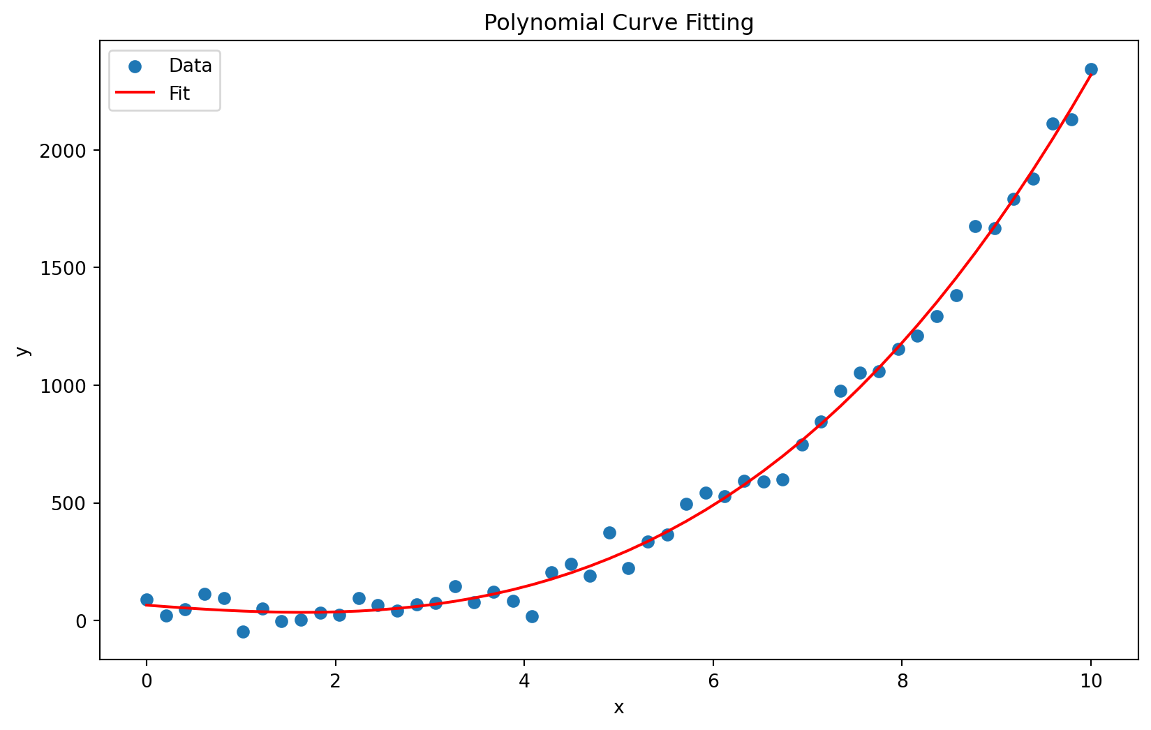
Example: fitting a polynomial

import numpy as np
import matplotlib.pyplot as plt

# Generate some noisy data points
np.random.seed(0)
x = np.linspace(0, 10, 50)
y = 2.5 * x**3 - 1.5 * x**2 + 0.5 * x + np.random.normal(size=x.size)*50

# Fit a polynomial curve to the data
coefficients = np.polyfit(x, y, 3)  # Fit a 3rd-degree polynomial
poly = np.poly1d(coefficients)
y_fit = poly(x)

# Plot the original data and the fitted curve
plt.figure(figsize=(10, 6))
plt.scatter(x, y, label='Data')
plt.plot(x, y_fit, color='red', label='Fit')
plt.xlabel('x')
plt.ylabel('y')
plt.title('Polynomial Curve Fitting')
plt.legend()
plt.show()

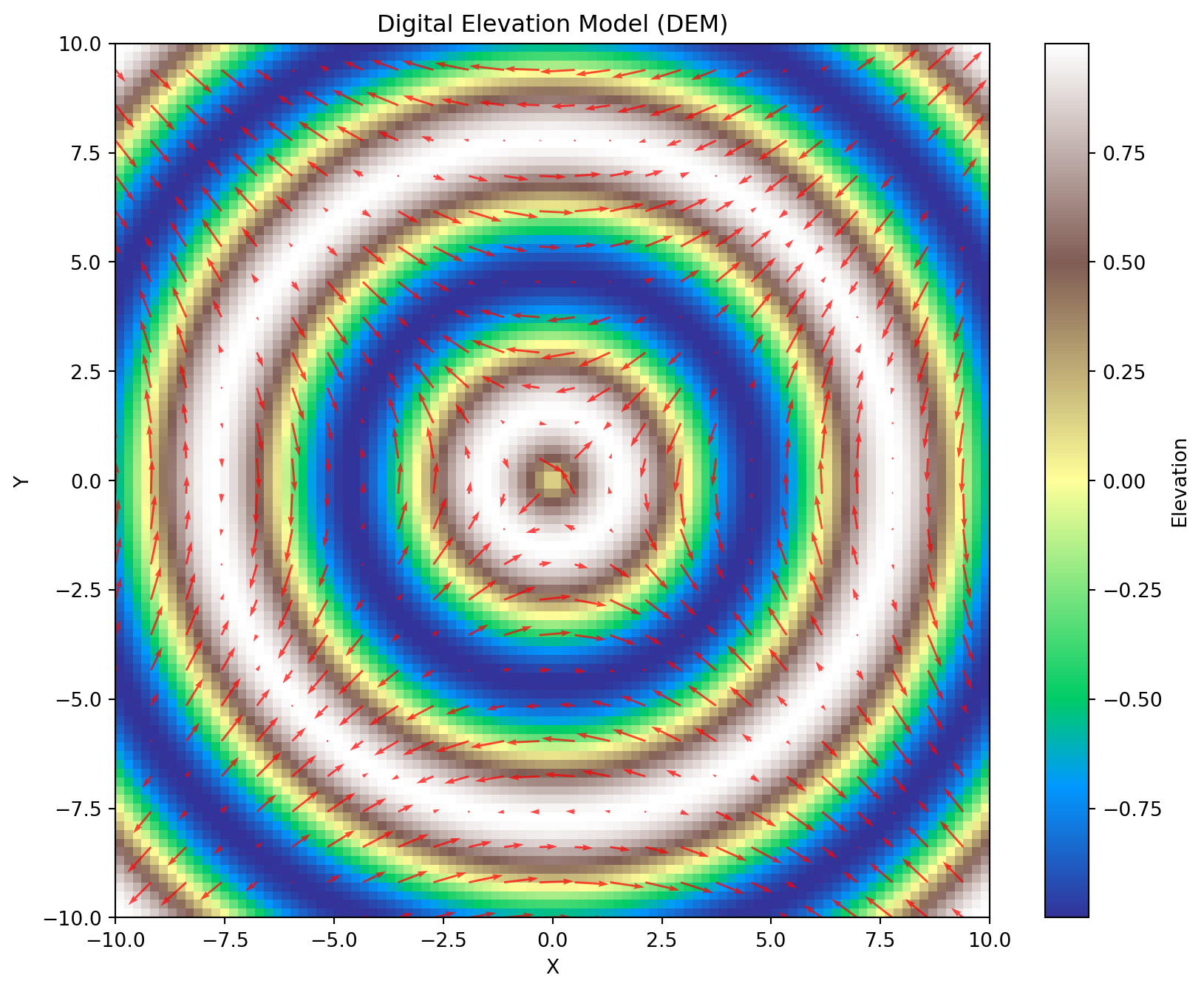
Example: a digital elevation model (DEM)

Given a DEM represented by a 2D NumPy array, the slope at each point can be calculated using the gradient method. The gradient method calculates the rate of change of elevation in the x and y directions, which can be used to determine the slope. This is very useful in many geoscience applications.

import numpy as np

# Sample elevation data (DEM)
x, y = np.meshgrid(np.linspace(-10, 10, 100), np.linspace(-10, 10, 100))
elevation_data = np.sin(np.sqrt(x**2 + y**2))
print(elevation_data)

# Calculate the gradients in the x and y directions
dx, dy = np.gradient(elevation_data)

# Calculate the slope magnitude
slope = np.sqrt(dx**2 + dy**2)

print("Slope at each point:")
print(slope)

[[0.99998766 0.99060935 0.96166494 ... 0.96166494 0.99060935 0.99998766]
 [0.99060935 0.96085316 0.9119285  ... 0.9119285  0.96085316 0.99060935]
 [0.96166494 0.9119285  0.8438217  ... 0.8438217  0.9119285  0.96166494]
 ...
 [0.96166494 0.9119285  0.8438217  ... 0.8438217  0.9119285  0.96166494]
 [0.99060935 0.96085316 0.9119285  ... 0.9119285  0.96085316 0.99060935]
 [0.99998766 0.99060935 0.96166494 ... 0.96166494 0.99060935 0.99998766]]
Slope at each point:
[[0.01326293 0.03539193 0.06266921 ... 0.06266921 0.03539193 0.01326293]
 [0.03539193 0.05563577 0.08247603 ... 0.08247603 0.05563577 0.03539193]
 [0.06266921 0.08247603 0.10790679 ... 0.10790679 0.08247603 0.06266921]
 ...
 [0.06266921 0.08247603 0.10790679 ... 0.10790679 0.08247603 0.06266921]
 [0.03539193 0.05563577 0.08247603 ... 0.08247603 0.05563577 0.03539193]
 [0.01326293 0.03539193 0.06266921 ... 0.06266921 0.03539193 0.01326293]]

In this example, we first calculate the gradients dx and dy in the x and y directions using np.gradient. Then, we calculate the slope magnitude at each point using the formula slope = sqrt(dx^2 + dy^2).

We can even use matplotlib to visualize the elevation and gradient:

plt.figure(figsize=(10, 8))
plt.imshow(elevation_data, cmap='terrain', origin='lower', extent=(-10, 10, -10, 10))
plt.colorbar(label='Elevation')
plt.title('Digital Elevation Model (DEM)')
plt.xlabel('X')
plt.ylabel('Y')

# Plot the gradient as quiver arrows
skip = 4
plt.quiver(x[::skip, ::skip], y[::skip, ::skip], dx[::skip, ::skip], dy[::skip, ::skip], scale=5, color='red', alpha=0.7)
plt.show()