In this exercise, we'll review basic Excel spreadsheets. Part B will extend this work to add charts.
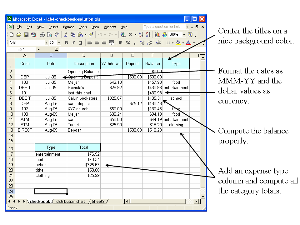
Begin by downloading this example spreadsheet: checkbook.xlsx. We'll try to make it look like this sample spreadsheet:
F3 that takes the opening balance from F2 and
subtracts the current withdrawal or adds the current deposit. When you've got the
formula, then copy it down the column. SUMIF formula to compute the values.
Use the function wizard to do this by
highlighting the expense type cell (C17 in the sample),
choosing the Formula tab, and then "Insert Function", searching for the function SUMIF,
clicking "OK", and then letting the function wizard walk you through the
process. After creating your formula with the wizard, your formula should look something like this:
SUMIF(a range indicating the checkbook type names,
      a cell indicating the type name condition,
      a range indicating the checkbook values to be summed)
(Hint: the two ranges from
the checkbook should start and end on the same rows.) When your
function is working, copy it down the column for each type category using the fill handle.
Remember to put commas between your 3 arguments and to use absolute and
relative references appropriately.This completes Part A of the check book exercise. DO NOT SUBMIT until you have also completed Part B. (You will be given time after Quiz 2 to work on Part B in class.)
We will grade this portion of the assignment according to the following criteria: