CS375 Week 4
Metrics and Loss Functions
Regression Metrics
- MAE: Mean Absolute Error (“predictions are usually off by xxx units”)
- MSE: Mean Squared Error (“predictions are usually off by xx units^2”)
- RMSE: Root Mean Squared Error (same units as the target)
- MAPE: Mean Absolute Percent Error (“predictions are usually off by yy%”)
- Traditional R^2 (fraction of variance explained)
MAE is like the median (cares about how many are above/below prediction); MSE/RMSE/R2 is like the mean (cares about the magnitude of errors)
All of these are also valid loss functions (i.e., we can use them to train a model).
Classification Metrics
- Accuracy: fraction of correct predictions
- If there’s just two classes (positive and negative), we can also compute:
- Precision: fraction of true positives among all positives
- Recall: fraction of true positives among all actual positives
- (Lots more metrics, especially for multi-class classification, or when we can freely set thresholds)
Partial Credit
- All regression metrics give partial credit for being close
- But not accuracy.
- So it’s hard to learn from mistakes
- Alternative: categorical cross-entropy (log loss)
Intuition: Predicting the outcome of a game
- Suppose you play chess grandmaster Gary Kasparov in chess. Who wins?
- Suppose you play someone with roughly equal skill. Who wins?
Answer as a probability distribution.
Good predictions give meaningful probabilities
- How surprised would you be if you played Gary Kasparov and he won?
- If you won?
- Intuition: surprise
Use surprise to compare two models
Suppose A and B are playing chess. Model M gives them equal odds (50-50), Model Q gives A an 80% win chance.
| Player | Model M win prob | Model Q win prob |
|---|---|---|
| A | 50% | 80% |
| B | 50% | 20% |
Now we let them play 5 games, and A wins each time. (data = AAAAA)
What is P(data given model) for each model?
- Model M:
0.5 * 0.5 * 0.5 * 0.5 * 0.5= (0.5)^5 = 0.03125 - Model Q:
0.8 * 0.8 * 0.8 * 0.8 * 0.8= (0.8)^5 = 0.32768
Which model was better able to predict the outcome?
Likelihood
Likelihood: probability that a model assigns to the data. (The P(AAAAA) we just computed.)
Assumption: data points are independent and order doesn’t matter. (i.i.d). So P(AAAAA) = P(A) * P(A) * P(A) * P(A) * P(A)
Log Likelihood
- Likelihood numbers can quickly get too small to represent accurately.
- Computational trick: take the logarithm.
- log2(.5) = -1 because 2^(-1) = 0.5
- log2((0.5)^5) = 5 * log2(0.5) = 5 * -1 = -5
- log of a product = sum of logs
Log likelihood of data for a model:
- Compute the model’s probability for each data point
- Take the log of each probability
- Sum the logs
Cross-Entropy Loss
- Negative of the log likelihood (“NLL”)
- Intuition: average surprise
- A good regression model predicts nearby the right answer.
- A good classifier should give high probability to correct result.
- Cross-entropy loss = average surprise.
Technical note: MSE loss minimizes cross-entropy if you model the data as Gaussian.
For technical details, see Goodfellow et al., Deep Learning Book chapters 3 (info theory background) and 5 (application to loss functions).
Categorical Cross-Entropy
Cross-entropy when the data is categorical (i.e., a classification problem).
Definition: Average of negative log of probability of the correct class.
- Model M: Gave prob of 0.5 to the correct answer. Cross-entropy loss = -log2(0.5) = 1 bit
- Model Q: Gave prob of 0.8 to the correct answer. Cross-entropy loss = -log2(0.8) = 0.3219 bits
(Usually use natural log, so units are nats.)
Math aside: Cross-Entropy
- A general concept: comparing two distributions.
- Most common use: classification.
- Classifier outputs a probability distribution over classes.
- Categorical cross-entropy is a distance between that distribution and the “true” distribution.
- Estimate the true distribution using a 1-hot vector with 1 in the correct class and 0 elsewhere.
- But it applies to any two distributions.
Future
Lab Review
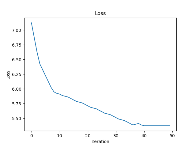
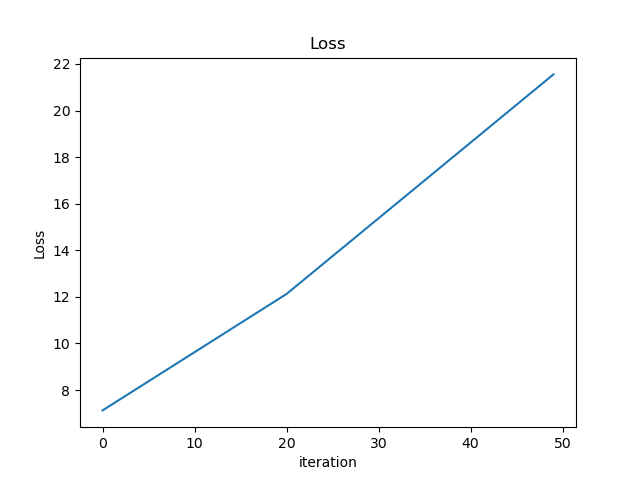
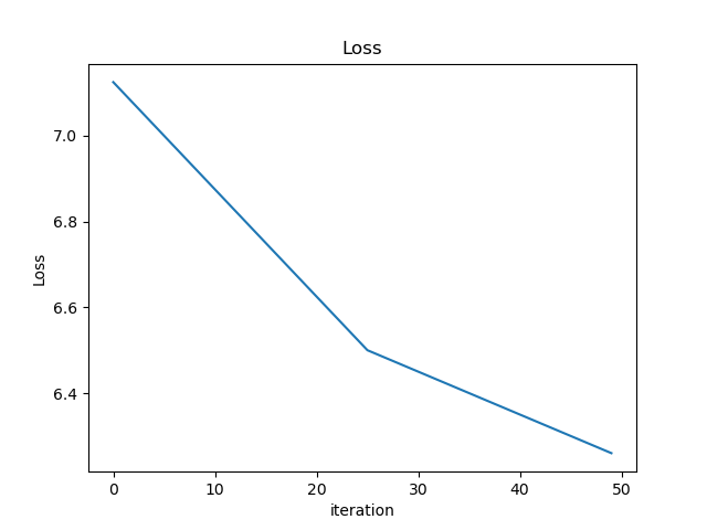
- Which of these plots of training loss is happiest? Why?
On the last step, we observed that the fitted model was different for MAE vs MSE. To get a different line, which had to change? (1) the computation of the loss, (2) the computation of the gradient, (3) both, (4) neither or something else.
If you changed how the predictions were computed, would you need to change how the loss function gradient is computed?
Takeaways
- Training curves should look like the one on the left:
- Often we train until convergence, i.e., loss stops going down (won’t be zero, might be noisy)
- The second one diverged (in this case, the gradient computation was incorrect, but you can also see this with too high learning rate, poor initialization, etc.)
- The third one was training too slowly (learning rate was too low); hadn’t yet converged.
- Gradients are the source of all learning in neural networks. What mattered wasn’t how the loss function was computed, but how its gradient was computed.
- Backpropagation is nicely modular: all computation happens locally, with only a small amount of communication (the gradients) between steps of the computation. It lets us break down the computation into small, automatable steps.
Think…
Can we use accuracy as a loss function for a classifier? Why or why not?
No, because its derivative is almost always 0.
Cross-Entropy vs Softmax
- How do we measure how good a classifier is? categorical cross-entropy loss
- Cross-entropy depends on probabilities, but the model gives us scores. How do we turn scores into probabilities? -> softmax
Review
Which of the following is a good loss function for classification?
- Mean squared error
- Softmax (generalization of sigmoid to multiple categories)
- Error rate (number of answers that were incorrect)
- Average of the probability the classifier assigned to the wrong answer
- Average of the negative of the log of the probability the classifier assigned to the right answer
Why?