CS 375 Review

Tuneable Machines Playing Optimization Games

Seeing but Not Perceiving

Go and tell this people:

“‘Be ever hearing, but never understanding;
    be ever seeing, but never perceiving.’
Make the heart of this people calloused;
    make their ears dull
    and close their eyes.
Otherwise they might see with their eyes,
    hear with their ears,
    understand with their hearts,
and turn and be healed.”

(Isaiah 6:9-10, NIV)

Quoted extensively in the New Testament (Matthew 13:14-15, Mark 4:12, Luke 8:10, John 12:40, Acts 28:26-27, etc.)

TODO: The point to make clearer: perception in Isaiah is purposive — seeing in order to “turn and be healed.” Contrast with models that “see” without purpose. We don’t just want to build machines that classify — we want to perceive with redemptive purpose, toward shalom. The passage warns against a kind of seeing that never arrives at understanding or action.

Tuneable Machines Playing Optimization Games

The Big Picture

We studied AI by building one from scratch: a neural network classifier.

Tuneable Machines (TM)

A computer made of tweakable math:

• Arrays of numbers flow through layers
• Each layer: multiply, add, squish
• Billions of knobs to adjust

Key deep-dive: the MLP classifier

Extension: the CNN we built for image classification = MLP but with convolutional layers in the feature extractor body.

Optimization Games (OG)

A game that defines what “better” means:

• A world where the agent can act and get feedback (e.g., dataset of labeled examples)
• A score function for quantifying success (e.g., loss)
• A strategy for improving (e.g., gradient descent)

Key deep-dive: supervised learning: mimicking a given set of (input, correct answer) pairs

This is the framing from week 1. The whole course has been about understanding both sides: what the machine computes and how we set up the game that teaches it. Each side has a core example we’ve studied in depth (the MLP, supervised learning) but also extends to other architectures and other games.

Part 1: Tuneable Machines

The MLP Classifier: Our Core Example

The simplest “deep” network — and the building block of everything else.

Input → [Linear] → [ReLU] → [Linear] → [Softmax] → Probabilities → Loss
 (784)    784→100            100→10

Every modern neural network is a variation on this theme: linear transformations, nonlinearities, and a loss function.

We built this up piece by piece across weeks 3-6. Start with linear regression (one layer, MSE loss), add softmax + cross-entropy for classification, add a hidden layer + ReLU for nonlinearity, and you have an MLP. The notebooks that trace this arc are u03-u06.

TM-LinearLayers: The Workhorse Operation

A linear layer computes y = x @ W + b:

• Matrix multiply (@): each output is a weighted combination of all inputs
• Bias (+ b): shifts the output
• “Fully connected”: every input connects to every output

# Manual:                        # PyTorch:
y = x @ W + b                    layer = nn.Linear(n_in, n_out)
                                 y = layer(x)

Shape rule: (batch, n_in) @ (n_in, n_out) → (batch, n_out)

Hands-on: u03n1 (manual linear regression), u04n3 (PyTorch logistic regression)

This is the most fundamental operation in neural networks. Everything else builds on it. The weight matrix W encodes “how much does each input feature contribute to each output.” The bias b shifts the decision boundary. The shape rule is the one thing students need to have deeply internalized.

TM-ActivationFunctions: Why Nonlinearity Matters

ReLU: y = max(0, x) — chop off the negative part.

Without it, stacking linear layers just gives another linear layer. With it, the network can learn conditional behavior: “activate this feature only when the input has this property.”

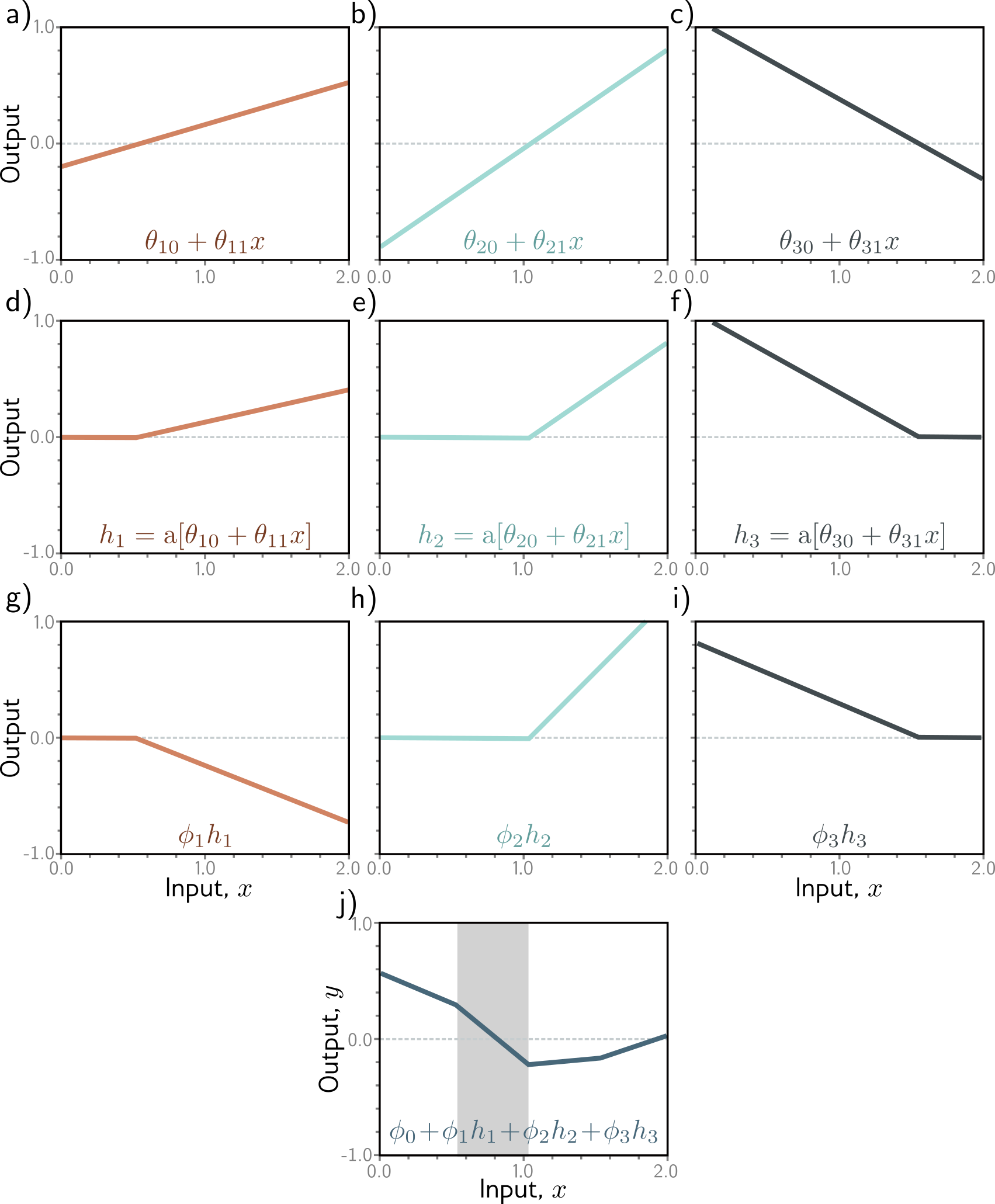
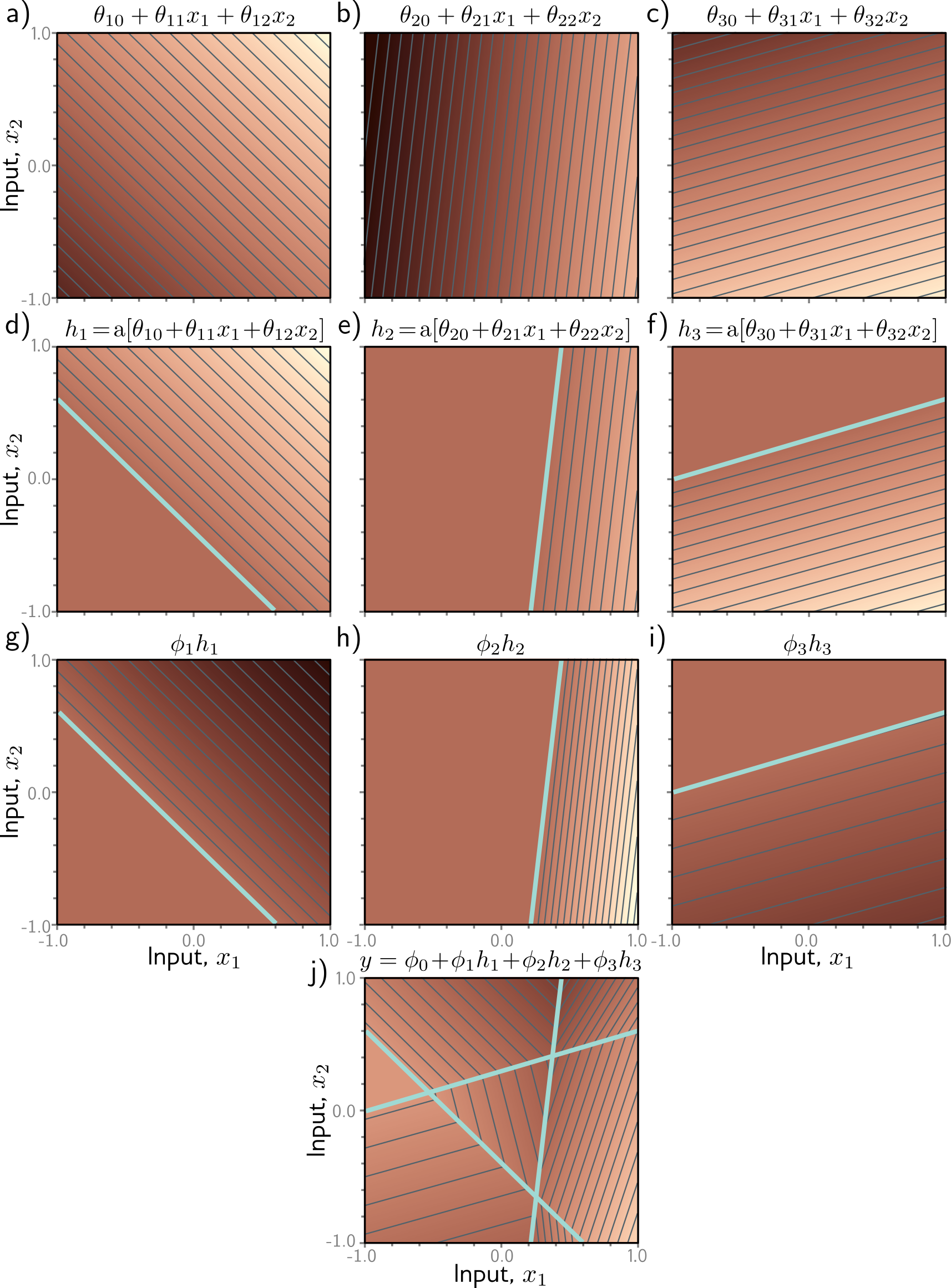
In practice, variants like GELU and SiLU/Swish avoid ReLU’s hard zero, giving smoother gradients. We use ReLU for simplicity; the intuition transfers.

Hands-on: u05n00 (ReLU interactive)

ReLU is the simplest nonlinearity and it’s used almost everywhere. The key insight: two linear layers composed are still linear (matrix multiply is associative). You need nonlinearity between layers for depth to matter. ReLU is preferred because it’s simple, doesn’t saturate for positive inputs, and gradients are easy to compute (1 or 0). The hard zero can cause “dead neurons” (a neuron that always outputs 0 never gets gradient signal), which is why modern architectures often use GELU (used in Transformers) or SiLU/Swish — these have a smooth curve near zero instead of a sharp corner.

TM-Softmax: Scores to Probabilities

Three steps: exponentiate → sum → divide.

logits:  [2.0,  1.0,  0.1]
exp:     [7.39, 2.72, 1.11]    (make positive)
softmax: [0.66, 0.24, 0.10]    (normalize to sum to 1)

• Largest logit (or “score”) → largest probability
• Adding a constant to all logits doesn’t change the output (but multiplying does!)
• Part of the architecture (we’d still use it even if the inputs happen to be valid probabilities)
• Paired with cross-entropy loss for classification

Hands-on: u04n2 (softmax), u05s2 (softmax deep-dive)

Softmax converts arbitrary real numbers into a valid probability distribution. It’s the final step in any classification network. The relationship with cross-entropy is important: cross-entropy measures “how surprised are we by the correct answer given our predicted probabilities?” PyTorch’s F.cross_entropy combines softmax + log + NLL for numerical stability.

TM-MLPParts: The Full Forward Pass

Given an image of a digit (flattened to a vector), compute the network’s prediction and loss:

1. Input vector (784,)
2. Layer 1: z1 = x @ W1 + b1 → shape (100,) — these are pre-activations
3. ReLU: a1 = max(0, z1) → shape (100,) — these are activations
4. Layer 2: z2 = a1 @ W2 + b2 → shape (10,) — these are logits
5. Softmax: probs = softmax(z2) → shape (10,) — these are probabilities
6. Loss: loss = -log(probs[correct_class]) — this is cross-entropy

We show one hidden layer; real networks stack many (repeating steps 2–3). The pattern is always: linear → nonlinearity → linear → nonlinearity → … → output.

Key vocabulary: weights, biases, activations, logits, probabilities, loss

Hands-on: u06n1 (trace MNIST classifier step by step)

Students should be able to trace through this by hand for a small example. The forward pass is pure computation — no learning happens here. Learning happens when we go backward (autograd) and update (optimizer). The distinction between parameters (W, b — learned) and activations (z, a, probs — computed fresh each time) is important.

TM-DotProduct: The Atomic Operation

The dot product of two vectors: multiply pairs, then sum.

a = [1, 0, 3]
b = [2, 5, 1]
a · b = 1×2 + 0×5 + 3×1 = 5

Three ways to think about it:

• Computation: it’s what matrix multiply does, element by element
• Similarity: high dot product = vectors point in similar directions
• Geometry: zero dot product = vectors are perpendicular (unrelated)

Caveat: dot product conflates direction and magnitude — a huge vector gets a high dot product with everything. Cosine similarity fixes this by normalizing to unit vectors first, isolating direction.

Hands-on: u04n1 (manual multi-output linear regression uses @ throughout)

TM-TensorOps: Shapes as the Type System

Shapes tell you what the data means:

• (batch_size, n_features) — a batch of feature vectors
• (n_features, n_classes) — a weight matrix
• (batch_size, n_classes) — predictions for a batch

The matmul shape rule: (m, n) @ (n, p) → (m, p) — inner dims must match.

Most bugs in neural network code are shape mismatches. Trace shapes through the network to debug.

Hands-on: u02n1 (PyTorch basics), u04n1 (multi-output regression)

Students should think of shapes like types in a programming language — they tell you what operations are valid and what the result will be. The batch dimension is always first. When shapes don’t match, the error message tells you exactly which dimensions disagree — read it carefully.

TM-DataFlow: Drawing the Diagram

          Parameters        Activations
          ──────────        ───────────
Input ──→ W1:(784,100) ──→ z1:(B,100)
(B,784)   b1:(100,)         │
                            ▼ ReLU
                           a1:(B,100)
                            │
          W2:(100,10)  ──→ z2:(B,10)    ← logits
          b2:(10,)          │
                            ▼ Softmax
                            probs:(B,10)    ← probabilities
                            │
          y_true:(B,)  ──→ loss: scalar  ← cross-entropy

• Parameters (W, b): learned, persist across batches.
• Activations (z, a, probs): computed fresh each forward pass.

Hands-on: u06n1 (trace MNIST), Quiz 2

How It Learns: Autograd

TM-Autograd: You write the forward pass; PyTorch computes the backward pass.

# Forward pass (you write this)
y_pred = model(x)
loss = F.cross_entropy(y_pred, y_true)

# Backward pass (PyTorch does this)
loss.backward()  # computes gradients of loss w.r.t. all parameters

# The gradient of each parameter tells you:
# "which direction would INCREASE the loss?"
# So we go the opposite direction.
optimizer.step()  # updates parameters to DECREASE loss

• requires_grad=True on parameters tells PyTorch to track operations
• loss.backward() walks the computation graph in reverse (chain rule)
• Gradients accumulate, so optimizer.zero_grad() clears them each step

Hands-on: u06n2 (compute gradients in PyTorch)

Autograd is what makes neural networks practical. Without it, we’d have to derive and implement gradients by hand for every architecture. The key insight: the forward pass builds a computation graph, and backward() walks it in reverse using the chain rule. This is the “backpropagation” algorithm — it’s just the chain rule applied systematically.

TM-Implement-TrainingLoop: The 5-Step Loop

for epoch in range(n_epochs):
    for x_batch, y_batch in dataloader:
        y_pred = model(x_batch)         # 1. Forward pass
        loss = loss_fn(y_pred, y_batch) # 2. Compute loss
        optimizer.zero_grad()           # 3. Backward pass
        loss.backward()                 # 
        optimizer.step()                # 4. Update parameters
    # 5. Evaluate on validation set
    val_loss = 0.
    for x_val, y_val in val_loader:
        with torch.no_grad():
          y_val_pred = model(x_val)
          val_loss += loss_fn(y_val_pred, y_val).item()

This is the same loop for every neural network — from MNIST to GPT.

Hands-on: u06n1 (MNIST in PyTorch), u06s2 (MNIST with augmentation)

OG-Theory-SGD: The Learning Mechanism

(Bridges both pillars: this is what connects the machine to the game.)

Gradient = direction of steepest increase of the loss.
Gradient descent = move parameters in the opposite direction.

• Learning rate: step size. Too big → overshoot. Too small → too slow.
• Stochastic (mini-batch): use a subset of data each step.
  • Faster than full-batch; noise helps escape bad local minima.

Parameters ──[subtract lr × gradient]──→ Updated Parameters

Beyond vanilla SGD:

• Momentum: accumulate past gradients to smooth updates and push through flat regions
• Adam: adapt the learning rate per parameter — no single learning rate fits all layers

Most practitioners default to Adam.

Hands-on: u03n1 (manual gradient descent for linear regression)

SGD is the optimizer behind all of deep learning. The gradient tells you which way is “uphill” for the loss, so you go downhill. Using random mini-batches instead of the full dataset is what makes it “stochastic” — this is faster and actually helps generalization because the noise prevents the model from settling into sharp minima that don’t generalize. Momentum is the easiest extension to motivate: a ball rolling downhill accumulates speed and can roll through small bumps. Adam combines momentum with per-parameter learning rate scaling, which is especially helpful when different parameters have very different gradient magnitudes (common in deep networks).

Beyond the MLP: Embeddings

TM-Embeddings: Neural networks represent data as vectors where geometric relationships encode meaning.

• Similar items → similar vectors (high dot product, small distance)
• Clusters in 2D visualizations show learned categories
• Learned embeddings capture structure that hand-crafted features miss

Examples: word embeddings (king - man + woman ≈ queen), image embeddings (CNNs), user/movie embeddings (recommender systems)

Hands-on: u07n1 (image embeddings), u09n1 (word embeddings - in 376)

Embeddings are arguably the most important concept for understanding modern AI. An LLM’s token embeddings, a search engine’s document embeddings, a recommender’s user embeddings — they’re all the same idea: represent things as vectors so that geometry captures meaning. Pretrained embeddings (like from a large CNN or LLM) are incredibly useful because they encode knowledge from massive datasets.

Beyond the MLP: Representation Learning

TM-RepresentationLearning: Hidden layers transform the data to make the task easier.

• Early layers: extract low-level features (edges, textures)
• Later layers: combine into high-level concepts (faces, objects)
• Final layer: a simple linear classifier on these learned features

This is why transfer learning works: the features learned for one task (ImageNet classification) are useful for many other tasks.

Hands-on: u05n1 (image classifier with pretrained feature extractor)

Beyond the MLP: Convolutions

Convolution: Specialized layers for spatial data (images).

Two key improvements over fully-connected layers:

• Parameter sharing: same small filter applied at every position
• Translation invariance: recognizes a feature regardless of location

A CNN = convolution layers + pooling + fully-connected layers at the end.

CNN Explainer interactive visualization: poloclub.github.io/cnn-explainer/

We didn’t go deep into CNNs, but the key ideas are important: parameter sharing dramatically reduces the number of parameters (a 3×3 filter has 9 parameters regardless of image size), and translation invariance means the network doesn’t have to re-learn what a cat looks like for every pixel position. Modern vision systems often use Vision Transformers instead, but CNNs are still widely used and the concepts transfer.

Part 2: Optimization Games

Supervised Learning: Our Core Game

The game has simple rules:

1. Given: a bag of (input, correct answer) pairs
2. Goal: learn to predict correct answers for new inputs
3. Score: how well do your predictions match? (loss function)

The machine learns by mimicry — imitating the training data.

This is the game we’ve played all semester. It’s deceptively simple to describe but rich in subtlety: What counts as a good loss function? How do we know the model works on new data? What happens when the training data doesn’t represent the real world? These questions drive the rest of Part 2.

OG-ProblemFraming-Supervised: Setting Up the Game

To frame a supervised learning problem:

1. Inputs: what does the model see? (features, images, text, …)
2. Targets: what should it predict? (numbers → regression, categories → classification)
3. Loss function: typically MSE for regression, cross-entropy for classification
4. Success metric: what do stakeholders actually care about?

Example: “Detect pneumonia from chest X-rays” → inputs = image, target = {pneumonia, healthy}, loss = cross-entropy, metric = sensitivity (TPR) — because missing a case is worse than a false alarm. Note: the loss (cross-entropy) is what the model optimizes; the metric (sensitivity) is what stakeholders care about. They’re often different!

Hands-on: u02n2 (sklearn regression), u03n2 (sklearn classification)

OG-LossFunctions: Keeping Score

MSE (regression): average of squared errors. Penalizes big mistakes heavily.

\[\text{MSE} = \frac{1}{n}\sum_i (y_i - \hat{y}_i)^2\]

Cross-entropy (classification): average surprise at the correct answer.

\[\text{CE} = -\frac{1}{n}\sum_i \log p(\text{correct class}_i)\]

Why not accuracy as a loss? Its gradient is almost always zero — the model can’t learn from it.

Hands-on: u03n1 (MSE by hand), u04n2 (cross-entropy), u04n3 (PyTorch classification)

The loss function is what defines the game. MSE says “be close to the right number.” Cross-entropy says “be confident about the right class.” Accuracy can’t be used for training because it’s a step function — a tiny change in weights almost never flips a prediction from wrong to right, so the gradient is zero almost everywhere. Cross-entropy gives smooth, informative gradients.

Playing the Game Well: Evaluation

OG-Eval-Experiment: Why held-out data matters.

• Training set: the model learns from this
• Validation set: we tune hyperparameters using this
• Test set: final, unbiased evaluation (touch it once!)

Learning curves (loss vs. epoch) tell the story of training:

• Loss goes down → learning is working
• Val loss goes up while train loss goes down → overfitting
• Both stay high → underfitting

Hands-on: every lab from u04 onward includes train/val curves

The fundamental insight: if you evaluate on the same data you trained on, you’re measuring memorization, not learning. The validation set is like a practice exam you haven’t seen. The test set is the real exam. Never tune hyperparameters on the test set — that’s like checking the answer key before the exam.

OG-Implement-Validate: Validation Discipline

Split before you fit. Always.

# 1. Split data FIRST
X_train, X_val, y_train, y_val = train_test_split(X, y)

# 2. Train on training set only
model.fit(X_train, y_train)

# 3. Evaluate on validation set
val_score = model.score(X_val, y_val)

# 4. Spot-check predictions on specific examples
model.predict(X_val[:5])  # Do these make sense?

Validation performance is a better estimate of real-world performance than training performance.

OG-Generalization: When Models Fail

Overfitting: model memorizes training data but doesn’t generalize.

• Symptom: train loss low, val loss high (or rising)
• Interventions: more data, augmentation, regularization (dropout, weight decay)

Underfitting: model can’t even fit the training data.

• Symptom: both train and val loss remain high
• Interventions: bigger model, more training, better features

Bias-variance tradeoff:

• Bias = error from wrong assumptions. A model that’s too simple consistently misses the pattern, no matter what training data you give it. (Think: fitting a line to a curve.)
• Variance = error from sensitivity to the specific training set. A model that’s too complex fits the noise in this particular sample and gives wildly different predictions on a different sample.
• The sweet spot balances both — complex enough to capture the pattern, simple enough not to memorize the noise.

Interactive: Bias-Variance · Double Descent (MLU Explain)

Hands-on: u06s1 (bias-variance), u06s2 (augmentation and regularization)

This is one of the most practically important skills: looking at learning curves and diagnosing what’s going wrong. The interventions are different for overfitting vs underfitting — using regularization on an underfitting model makes things worse. Data augmentation is often the best first move for overfitting because it’s free and usually helps. The double-descent link is a bonus for curious students: at extreme overparameterization (more parameters than data points), test error can decrease again after the classical overfitting peak. This is surprising from the classical bias-variance perspective but is well-documented in deep learning.

OG-DataDistribution: Training ≠ Deployment

The model can only learn what’s in the training data.

• Selection bias: training data missing certain groups or conditions
• Domain shift: deployment conditions differ from training (time, geography, demographics)
• Data augmentation: artificially expand the distribution (flips, crops, noise)

A model that’s 99% accurate on ImageNet may fail on photos from a different camera, lighting, or culture.

Hands-on: u06s2 (augmentation), HW1 (real-world image classification)

This connects to the ethics discussions. When a facial recognition system works well on light-skinned faces but poorly on dark-skinned faces, that’s a data distribution problem — the training data was biased. Data augmentation helps but can’t fix fundamental gaps. Students should always ask: “Who is in the training data? Who isn’t?”

Beyond Supervised: Other Games

OG-ProblemFraming-Paradigms: Not all learning is mimicry.

Paradigm	Learning signal	Example	What it can learn
Supervised	Labeled examples	Image classification	To imitate the labels
Self-supervised	Predict hidden parts of data	GPT (predict next token)	Patterns in data
Reinforcement	Rewards from interaction	Game playing, robotics	Strategies beyond imitation

• Supervised learning is limited to imitating the training data.
• RL can explore and discover strategies no human demonstrated. It builds its own training data by trying things and seeing what works.

Self-supervised learning is what makes LLMs possible — you don’t need human labels, just lots of text. The model learns to predict what comes next, and in doing so learns grammar, facts, and reasoning patterns. RL is how AlphaGo discovered moves no human had played. The tradeoff: RL needs interaction (expensive), while supervised learning just needs a dataset.

Beyond Supervised: Pretrained Models

OG-Pretrained: Standing on the shoulders of giants.

The body + head pattern:

[Pretrained feature extractor] → [Your task-specific classifier]
       (frozen or fine-tuned)         (trained from scratch)

• Benefits: leverages knowledge from massive datasets; works with small task-specific data
• Risks: inherited biases, domain mismatch, licensing
• Fine-tuning vs. feature extraction: update the body or freeze it?

Hands-on: u05n1 (pretrained CNN for image classification), HW1

This is how most practical ML works today. You rarely train from scratch. A pretrained CNN (like EfficientNet trained on ImageNet) gives you excellent image features. A pretrained LLM gives you excellent text features. You just need to train a small head for your specific task. The question of when to fine-tune vs freeze depends on how similar your task is to the pretraining task and how much data you have.

LLM APIs: Using sequence models

response = client.chat.completions.create(
    model="gpt-5.2",
    messages=[
        {"role": "system", "content": "You are a helpful assistant."},
        {"role": "user", "content": "Classify this review as positive or negative: <review>..."}
    ]
)
result = response.choices[0].message.content

• Key abstraction: the conversation — a structured “document” with system instructions, user messages, assistant responses, “tool” calls/responses, reasoning traces

• API: you ask for the next message given the conversation so far (no training)

• Stateless: Each conversation is independent — the model itself doesn’t remember past conversations (but system can prepend them to future conversations)

• Agent extension: the model can output requests to run code (e.g., search, calculate, edit file); the system runs the code and includes the output in the conversation

• When appropriate: text tasks, prototyping, when training data is scarce

• When not: latency-critical, cost-sensitive, tasks requiring precise numeric output

LLM APIs are supervised learning taken to an extreme: someone else trained a massive model on internet-scale data, and you get to use it via an API. The system/user message structure lets you frame your task. This is a different kind of “optimization game” — you’re not training, you’re prompt-engineering. But understanding how the model was trained (self-supervised pretraining + RLHF) helps you use it better.

Part 3: The Bigger Picture

Overall: Context and Implications

We’ve studied the mechanics. Now: what does it mean?

The Overall objectives are about stepping back from the technical details and asking bigger questions. Some of these we addressed directly in class discussions and readings; others are more about the dispositions and habits of mind you’ve been developing throughout the course.

Overall-Impact: Who Is Affected?

When deploying an AI system, ask:

• Stakeholders: Who benefits? Who might be harmed? (Often different groups.)
• Distribution: Does the training data represent the deployment population?
• Feedback loops: Will the system’s outputs change future inputs?
  • Resume screening → fewer diverse hires → less diverse training data → …
  • News recommendations → users see only confirming views → more extreme content → …
• Recourse: What happens when the system is wrong?

(based on Shneiderman, Human-Centered AI; see also Gender Shades, COMPAS; ACM FAccT

This is the objective we addressed most directly. The case studies from w07 are good reference points. The key skill is going beyond “is this system accurate?” to ask “accurate for whom? at what cost? with what second-order effects?” Feedback loops are especially insidious because they make biases self-reinforcing.

Overall-Faith: AI in God’s Story

Christian concepts that inform how we think about AI:

• Imago Dei: humans are made in God’s image — AI capabilities don’t diminish human dignity
• Shalom: technology should contribute to wholeness, not just efficiency
• Stewardship: we’re responsible for how we build and deploy these tools
• Imitation: Paul urged Christians to imitate Christ — what does it mean when machines imitate us? Act like you want the machine to imitate you when it counsels others.

“We shape our tools, and thereafter our tools shape us.” — Churchill/McLuhan

This isn’t about having the “right answer” — it’s about genuine engagement. Can you articulate how a specific Christian concept changes how you’d approach a specific AI application? For example: “Imago Dei means a hiring algorithm shouldn’t reduce people to a score” or “Stewardship means we’re responsible for the biases our model inherits.”

Connections

Looking Forward to CS 376

Building state-of-the-art AI systems out of the building blocks we’ve studied:

• Flexible data structures: architectures for text, images, sound, etc. (e.g., attention, transformers)
• Generative models: producing images, text, audio
• Advanced use of LLMs: prompting, RAG, tool use, agents
• Reinforcement learning: learning from exploration and experience
• The training pipeline: how models like DeepSeek are actually trained

Optimizing the Right Thing

• Goodhart’s Law: “When a measure becomes a target, it ceases to be a good measure.”
• Example: optimizing for clicks → clickbait; optimizing for accuracy → gaming the test set; optimizing for engagement → social media addiction
• We’ve built amazing machines for optimizing numbers at huge scale.
• Is it good to optimize that number?
• AI will eventually “game” even the best-intentioned measures.
• Need people who can reflect on how numbers do/don’t reflect values.

Human Futures

• Everything that:
  1. Has a clear metric of success
  2. Can be done sitting alone at a computer (including operating a robot)
  3. Is repeatable
• will be automated sooner or later. So you should emphasize:
  • Situations where “good” is hard to define
  • Incarnate in the world, in community
  • Being vulnerable and courageous

Remind you of Calvin’s mission?

We are not machines. That’s good. Don’t forget it.

Reflection

What concept from this course has changed how you think about AI?

What questions do you still have?

Commission

Whatever you do, work at it with all your heart, as working for the Lord, not for human masters, since you know that you will receive an inheritance from the Lord as a reward. It is the Lord Christ you are serving. — Colossians 3:23-24

Treat people as God’s image-bearers, not like machines.

Work with AI systems, not as magic but as computational tools.

Keep learning. Keep thinking. Use the natural intelligence God gave you, together with all the artificial intelligence that God enabled, to love God and neighbor.