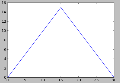
f(x) = maximum/2 - abs(maximum/2 - x)
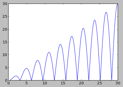
f(x) = abs(x * sin(x))
In this lab exercise, you’ll work with the AIMA Python implementations of local search algorithms.
In local search, we’d like to find the maximum value for a given objective function. Consider the two functions shown here. There’s no particular magic in either of them; they simply generate a set of objective values in two dimensions (only) that are all positive and display interesting global and local maxima:
f(x) = maximum/2 - abs(maximum/2 - x) |
f(x) = abs(x * sin(x)) |
These plots were created with Matplotlib by this script: graphs.py.
Local search algorithms work with complete-state formulations.
Download and run this Absolute value variant module and answer the following questions:
exp_schedule()
method in the simulated annealing function call?
That objective function wasn’t that interesting. Let’s try a slightly more interesting one, still in two dimensions.
Create a new module, similar to the absolute value variant from exercise 3.1, that uses the sine function variant specified above as its objective function. Get your new implementation running and then answer the following (similar) questions:
delta)
affect the operation of the two algorithms? Why or why not?
Because local search algorithms can hit local minima, it is useful to run them more than once or to run them in parallel.
Add code to implement random restarts for the abs-sin function, that is, run each algorithm multiple times with random initial states.
One key advantage of local search is the reduced memory requirements. This can be leveraged to allow more than one state to be maintained in parallel.
Consider the use of local beam search in which the successor states are chosen using one of the two algorithms as applied to the abs-sin function.
The text discusses Local beam search in Section 4.1.3, generally assuming that successor states are chosen using simple hill-climbing.
Submit the files specified above in Moodle under lab 3.