This page will become an outline of the entire class.
Note: this page includes a substantial amount of text generated by GitHub Copilot, mostly in the form of either (1) fleshing out an outline that I’d written or (2) explicitly stating some of the implications and details that are obvious to me but, I realized from the Copilot suggestion, might not be obvious to students. I would love to be able to credit the original sources for the material that it retrieved, but this use case has not been emphasized by those developing the underlying technology; see my blog post on gratitude. Note that there is an ongoing class-action lawsuit against GitHub Copilot around this issue; my hope is that this lawsuit helps encourage the development of pro-gratitude technology. Perhaps this hope is overly optimistic.
Unit 1: Introduction
Overfitting as a problem?
The figure in the book is misleading.
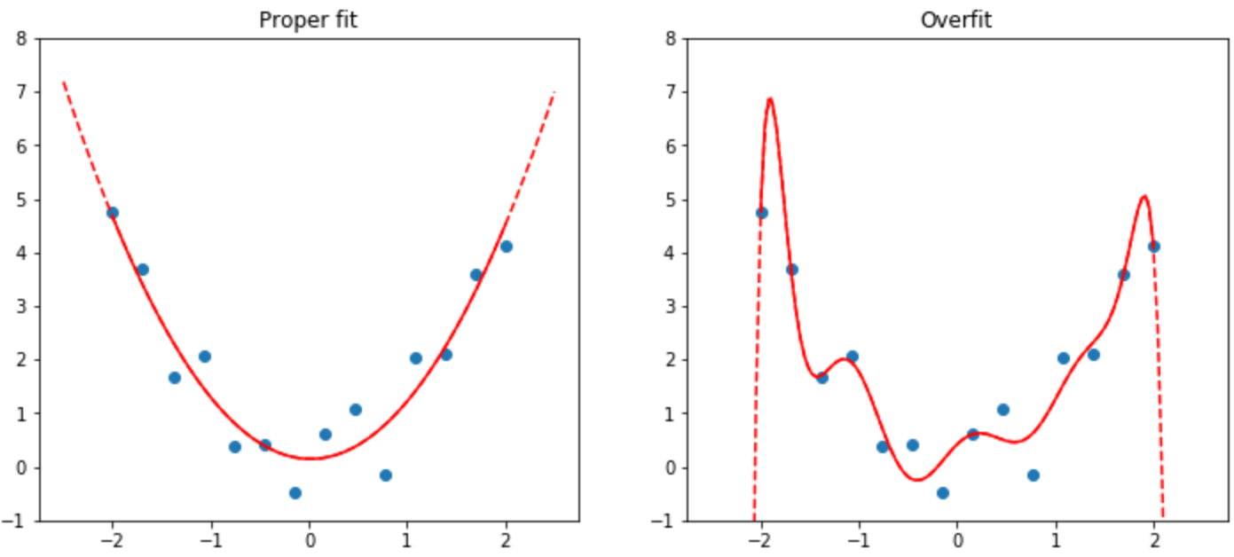
- That’s a polynomial fit. It’s much more sensitive than the functions typically used in NN’s.
- Recent results: a model can completely memorize its training set while still generalizing well (its behavior away from training set points is typically much better behaved than the figure suggests!), and in fact continue to improve generalization performance after reaching 100% accuracy (e.g., Grokking paper).
- Early stopping might hurt because of “double descent”.
- So yes, overfitting can be a problem, but don’t angst over it, just keep training.
- But: memorization might be a problem. “Phone: xxx-yyy-zzzz. SSN: "
There’s also underfitting. Underfitting means that the model isn’t capturing the patterns even of the training data. It usually means that your model is too small (so the range of functions it can approximate isn’t rich enough), or your training is insufficient (your learning rate is too low, you’re not giving it enough time to train, there’s something broken about the training process, etc.).
Why Python?
- Many libraries: talk with databases, webservers, IoT, GUIs, etc.
- Particularly good scientific computing ecosystem (NumPy, SciPy)
- Readable!
- Flexible: Enough metaprogramming to be concise where needed; some limited amount of magic is possible.
- Fast enough. Core operations are in low-level code; Python is the conductor.
- Array programming
- Benefits of GPU: highly parallel. Good for array operations (matrix multiply, nonlinearity, softmax)
- Computer graphics often requires doing nearly the same sequence of operations to lots of polygons and ending up with lots of pixels. Analogously, machine learning often requires doing nearly the same sequence of operations to lots of numbers. So hardware that was designed to do graphics well has been repurposed to do machine learning well too.
- GPU hardware has been adapted to be better suited for machine learning too, e.g., the addition of tensor cores.
Lots of jargon!
The more often something shows up in class, the more important it is to know.
Do we need math?
Yes! But not all at once. Some highlights:
- Linear algebra: vectors, linear operators (matrix multiplication), dimensionality reduction
- Calculus: chain rule
Can we explore the validation set, or should we leave it totally hidden?
To get some assurance about how our model will work once deployed, we need some data that we intentionally don’t look at until the very end. That’s the test set. But we often need to guess at how well it’s going to work before then—e.g., because we’re adjusting a parameter that might affect how well the model generalizes. The validation set (or, sometimes, validation sets) help us estimate that.
In general, it’s a good idea to look at the validation set to understand how and why the model worked or didn’t, e.g., get an overview of what kinds of images an image classifier tends to misclassify. But it’s probably not a good idea to study it in too much depth, or it will stop being a good proxy for the test set.
What if the randomly selected held-out part was the most unhelpful?
(Note: validation of 20% means training set is 80%.)
- This is why we need sizeable validation sets. (What if it happened to pick only the easiest examples for validation?)
- Randomness usually helps: it’s pretty unlikely to randomly select all extreme examples
- But do audit your choices, especially when summary stats may hide issues, e.g., unusually poor performance for a minority.
What are layers? What does each one do?
Gradually integrating information from wider area of the image. Lower layers = really zoomed in.
Converting sound to image is a cool idea.
Recently this approach has been replaced by: turn everything into a sequence and pretend it’s language.
Pretrained models are useful.
But can introduce bias, may not actually be as helpful as thought (more later).
How might we prove the universal approximation theorem?
- Specific theorems vary, but generally: any two linear transforms with a nonlinearity in between can approximate an arbitrary function.
- Intuitively, think about representing a single-variable function by piecewise lines (that’s basically a ReLU approximation, as we’ll study.)
- More generally, you can approximate any function by gradually refining a mesh and interpolating between the points.
- Beyond that, see the Wikipedia page and citations there.
How to collect data?
- Lots of preexisting datasets
- Logs from your website, app, IoT
- Crowdsource labels
AI libraries?
- PyTorch vs TensorFlow: very similar; historically Tensorflow more industry and PyTorch more research but that’s less clear now
- Keras, fast.ai, PyTorch Lightning: high-level libraries for making common patterns fast in TensorFlow and PyTorch
- newcomer: JAX. Simple automatic differentiation layer (autograd) on top of hardware-accelerated linear algebra primitives (XLA). Google.
Epoch?
One full pass through the training data. Not uncommon to see tens or hundreds of epochs, depending on training set size.
SGD?
- Gradient descent: which little wiggle would improve performance on the whole dataset?
- SGD: which would improve performance on these few images I just saw?
- SGD gets to a better solution faster than complete gradient descent. (intuition: more chances to try something and get feedback.)
Unit 2
General
- Your notebooks should generally make sense when read top to bottom. So:
- Use Markdown cells to narrate what you’re doing, and for narrative answers (like the rule for Jupyter cell output).
- Intersperse Markdown cells with corresponding code, so you don’t have to scroll up and down to match things up.
- Write narrative answers in complete sentences, so you don’t have to look at the questions to understand the answers.
- I suggest one response per cell; start each response with a
**bold**micro-heading, e.g.,**accuracy**: My classifier achieved accuracies between 75% and 100%.
- I suggest one response per cell; start each response with a
- Read it before you submit it.
- We’ll get to the low-level details that matter soon, so:
- Don’t worry that you don’t know all the low-level details of how classifiers work, e.g., what all the numbers do. We’re gradually peeling back layers over the next few weeks.
- Don’t worry about not knowing the low-level details of how to make fastai
DataLoaders. That’s not a learning objective of this class.- If you understand what the data loaders give you (batches of numbers paired with labels), you’re set.
- I’ve had to look up things in the tutorials and docs; see, e.g., Homework 3.
- Be clear what the notebook output rule is: the value of the last expression in the cell. (Assignments aren’t expressions.) It also shows the result of any
print(),display(), or plotting.- Instead of
print()ing outputs, leverage the notebook cell output rule: just put the variable name on the last line of the cell. e.g.:resid = y_true - y_pred resid
- Instead of
show_batchshows the labels, not the model’s predictions. (for that you canshow_predictions.)
Image Tensors
- The image tensor is batch by color channel by height by width. (I may have width and height flipped, can someone check this?)
- batch: the number of images in the batch.
- color channel: 3, one for each of red, green, blue (RGB). It’s as if each image is actually 3 images, one for each color channel.
- Manipulations
1.0 - imageinverts the colors in the image: black goes to white, etc.- This broadcasts across all of the numbers in the tensor.
- It’s as if we’re subtracting from an image tensor of the same shape but just filled with 1s.
Random Numbers
- The numerical value of the seed is unimportant and should not be reported in narrative. It just “throws the dice” again.
Reflections on Homework 1
-
Sideways images: fastai doesn’t honor EXIF orientation flags. I submitted a bug report.
-
What effect would burst photos have?
-
Accuracy numbers: why might we see the exact same accuracy number from several different variations of classifier hyperparameters, etc.?
-
Include stats about your dataset, e.g., how many photos total?
-
What choices did you make in your data collection?
- Who wrote the letters?
- What tool did they use? (pen? pencil? crayon? stylus? mouse?)
- What was the background color?
- What other things are on the images? (ruled lines on the paper? other letters?)
-
What choices did you make in the modeling?
- Size of the images? (
Resize) - What base model (
resnet18,resnet34, etc.)? - What batch size?
- Did you end up leaving out any images because they didn’t fit into a batch?
- How many epochs?
- What learning rate?
- Any data augmentation?
- Size of the images? (
Unit 5
This section contains text generated by GitHub Copilot, an AI.
Classification = scores (from linear layers), transformed to probabilities via softmax, trained to optimize cross-entropy loss.
Classification Diagram
note: scores are more commonly called logits.
Models
- For logistic classification (commonly but confusingly called logistic regression),
model = nn.Linear(in_features, out_features, bias=True). - For an MLP (Multi-Layer Perceptron) with a single hidden layer of
n_hiddenhidden features and ReLU activation:
model = nn.Sequential(
  nn.Linear(in_features, n_hidden, bias=True),
  nn.ReLU(),
  nn.Linear(n_hidden, out_features, bias=True)
)
Basic Implementation of a Classifier
We do the normal training loop: for batch, labels in dataloader:. Inside the training loop:
logits = model(batch)
probs = F.softmax(logits, axis=1)
loss = F.nll_loss(probs, labels)
# Or, better replacement for the above two lines:
# loss = F.cross_entropy(logits, labels)
# F.cross_entropy is a PyTorch function that combines the softmax and the negative log likelihood loss
# it is faster and more computationally stable.
loss.backward()
optimizer.step()
model.zero_grad()
We also usually want to keep track of our metrics. So we might do:
prediction = logits.argmax(axis=1)
num_correct_this_batch = (prediction == labels).float().sum()
num_correct += num_correct_this_batch
- Logistic regression
model = nn.Linear(n_input_features, n_classes).- That is, the model is a single linear layer.
- Its weight matrix is
n_input_featuresbyn_classes. - Its bias vector is
n_classeslong.- It adds a fixed amount to each class score, to allow us to model some classes as being just more likely than others a priori.
Metric vs Loss
- Metric: a number that tells you how well your model is doing. (e.g., accuracy)
- Loss: a number that tells you how well your model is doing, but is used to train the model. (e.g., cross-entropy loss)
- Why do we need both? Because we want to know how well our model is doing, but we also want to train it to do better.
- Why not just use the loss? Because the loss is not always a good metric. For example, if you’re ultimately trying to make a decision, you might want to optimize for accuracy (or a related measure like false-positive rate), not cross-entropy loss.
- Why can’t we train using a metric? Because metrics are not differentiable. (e.g., accuracy is not differentiable.) The gradient of accuracy with respect to any of the model parameters is always zero, so the model can’t learn anything.
Cross-entropy loss
Negative logarithm of the probability of the correct class. (For classification problems.)
Let $y_i$ be the correct class for the $i$th example in a batch. Let $p_i$ be the probability of that class, as computed by the softmax function. Then the cross-entropy loss for that example is $-\log(p_i)$. The cross-entropy loss for the whole batch is the average of the losses for each example.
- Can be thought of as “surprise”
- Like MSE, lower is better.
- How to get lower? Be confident in the right answer, and not confident in the wrong answers.
- How to compute it, for a classification setting?
- Compute the classifier’s scores for each class.
- Convert them into probabilities (usually by softmax)
- Look up what the right answer was (which class it should have been).
- Look up what probability the classifier gave to that class.
- Compute the negative logarithm of that probability.
- Do this same thing for all the examples in the batch; average the results.
- Why do we take the logarithm?
- Intuition 1: information theory.
- If there were 2 classes, but we had no information about which class it was, we’d learn 1 bit of information from finding out what the right answer was.
- If there were 4 classes, but we had no information about which class it was, we’d learn 2 bits of information from finding out what the right answer was.
- The pattern: we learn log2(number of classes) bits of information from finding out what the right answer was – if we had no prior idea what the right answer was.
- That’s the loss: how uncertain we were about this example.
- If we were 100% certain (and right), we’d learn 0 bits of information.
- The better the classifier, the less uncertain we are about the right answer.
- Intuition 2: product of probabilities
- The probability of two independent events is the product of their individual probabilities.
- But products are hard to deal with
- So it’s easier to work with sums of logs.
- An average is just a sum divided by the number of things being averaged.
- Intuition 3: expected message length.
- Intuition 1: information theory.
- Units: bits (if the log is base 2), or nats (for log base e).
- A bit is just ln(2) (about 0.7) nats.
- A nat is just log2(e) (about 1.4) bits.
- So they’re the same thing, just in different units.
Aside: cross-entropy is a general idea, not just for classification. For example, MSE for a regression problem can be viewed as a cross-entropy loss, where we view the model as predicting the mean of a distribution with constant variance. Maximizing the likelihood is the same as minimizing cross-entropy.
Softmax
A way to turn scores (unconstrained) into probabilities (nonnegative, sum to 1).
$$\text{softmax}(scores) = \frac{\exp{score_i}}{\sum_j \exp{score_j}}$$
- Remember the two rules for probabilities:
- All probabilities are between 0 and 1.
- The sum of all probabilities is 1.
- Scores might be negative, or positive, or both, and they probably don’t sum to 1, so we can’t use them as probabilities.
- But we can fix both problems:
- Subtract the largest score from all the scores, so the largest score becomes 0. (optional, but we’ll see why it’s useful later.)
- Take the exponential of each score, so all the scores are positive.
- Divide each score by the sum of all the scores, so the sum of all the scores is 1.
- So now we have a function that takes scores and gives probabilities, and it satisfies the two rules for probabilities.
- This function is called
softmax.- In math notation,
softmax(x)is writtenexp(x) / sum(exp(x)). expis the exponential function, e.g.,exp(1) == e.- In code,
softmax(x)is writtenexp(x) / exp(x).sum(). - In PyTorch,
softmax(x)is writtenF.softmax(x, dim=1)(wheredim=1indicates which axis has the scores for each class).
- In math notation,
- Numerical aside: Why do we subtract the largest score?
- If we don’t, then the largest score might be so large that the exponential overflows.
- So we subtract the largest score, so the largest score becomes 0, and the exponential doesn’t overflow.
- This is a common trick in numerical computing: subtract the largest number to avoid overflows.
- This works because you can add or subtract a constant from the input to
softmaxwithout changing the output. (exercise to the reader: prove it!)
- Logits vs logprobs
- The model’s output is called the logits, which is a vector with one number for each class.
- Usually they’re the result of a Linear layer, so they’re not constrained to be probabilities.
- We interpret each logit as the log of the unnormalized probability of each class. (hence the name)
- To normalize the probabilities, we could apply
softtmaxand then take the log of the result. Butlog(softmax(x)) = log(exp(x) / sum(exp(x))) = x - log(sum(exp(x))). So we can just subtract the log of the sum of the exponentials of the logits, and we get the same result. This is called the The Log-Sum-Exp Trick.
Additional resource: Softmax for neural networks
Where do scores come from?
- How does the classifier compute scores?
- A linear regression for each class
- So each score is the dot product of the input with the weights for that class.
- So, intuitively, the classifier is measuring how similar the input is to each class, and then converting those similarities into probabilities.
- How do we know what was the right score?
- In linear regression we were given the right scores.
- In classification, we have to learn the scores from data. (hence Elo scores)
Why nonlinearities?
- Remember we’re trying to fit a function from inputs to outputs.
- The function is a model.
- The inputs are the (training) data.
- The outputs are the labels.
- A wide range of interesting problems can be expressed as a function from inputs to outputs.
- Example: classifying an image. The inputs are the pixels, and the outputs are the probabilities of each class.
- Example: predicting the price of a house. The inputs are the features of the house, and the outputs are the price.
- Example: predicting the next word in a sentence. The inputs are the previous words, and the outputs are the probabilities of each word.
- Without nonlinearities, the model is just a linear regression.
- Linear regression is not powerful enough to learn anything interesting.
- So we need nonlinearities to make the model more powerful.
- Example nonlinearity: the rectifier (ReLU)
- other examples: sigmoid, tanh, leaky ReLU, etc.
- ReLU is the most common (and simplest)
- Why is ReLU useful?
- We can approximate any function as a piecewise linear function.
- It’s easiest to see this with a 1D function, as we started to see in last week’s lab.
- But it’s true for any number of dimensions.
- We can make any piecewise linear function we want by combining ReLUs.
- So we can approximate any function we want by combining ReLUs.
- We can approximate any function as a piecewise linear function.
- The same applies for other nonlinearities also.
Unit 6
- Pre-training and fine-tuning
- Pre-training tasks
- classical: ImageNet
- modern: self-supervision
- How to fine-tune
- Give the model a new “head”
- Train just the new head
- Train the whole model end-to-end
- Pre-training tasks
- What heads can we use?
- Classification heads
- To softmax or not to softmax?
- Binary vs Categorical Cross-Entropy
- The fast.ai book isn’t clear here.
- When the task is pick which one of these N classes applies to this example, the classifier’s output for each example is a category probability distribution over the N classes.
- So the output is a vector of N probabilities that sum to 1.
- So we use softmax to ensure that the output is a valid categorical distribution (i.e., the probabilities are nonnegative and sum to 1).
- And we use (categorical) cross-entropy to measure the loss: negative log of the probability of the correct class.
- When there are only two classes, we can use a single number instead of a vector of two numbers. (We just pretend that the other class has a score of 0, and everything works out the same.)
- So the output is a single number, -inf to inf, corresponding to the score of the “positive” class.
- We imagine that the score for the negative class is zero. So positive scores mean evidence in favor of the positive class, and negative scores mean evidence in favor of the negative class.
- The classifier’s output for each example is a Bernoulli distribution over the two classes.
- We still compute the cross-entropy loss, but the code is simpler because we’re only dealing with a single number.
- When we’re doing multi-label classification, the book’s approach is actually to treat this as a bunch of separate binary classification problems.
- So we have a separate classifier for each label.
- Each classifier’s output is a single number, -inf to inf, corresponding to the score of whether the image has that label.
- The
BCEWithLogitsLossloss function will conveniently compute the loss across both dimensions (for each example, for each label) and compute the average.
- Regression heads
- Loss functions
- We can also use MAE or MAPE
- Loss functions
- Classification heads
- Making models generalize better
- Augmentation: make your training data more diverse
- Intuition: carefully studying past exams.
- What if you say: ‘When the question includes the letter “m”, the answer is always “B”.’
- That’s much easier to learn than how to think through solving the question.
- So it leads to higher confidence in answers for practice exams.
- Regularization: avoid excesses
- excessive use of individual features
- problem: might overfit to the training data
- solution: penalize large weights
- excessive confidence in predictions
- problem: might overfit to the training data, even mistaken labels
- solution: penalize probabilities that are too close to 0 or 1.
- excessive use of individual features
Unit 7
Recommender Systems
(no Copilot in this section)
- Classical approach:
- manually annotate every item with metadata (e.g., highly nuanced movie genres)
- user says what genres they like, get a ranked list of movies.
- but: tedious for platform and user, doesn’t capture nuances.
- Collaborative Filtering approach
- uses only interaction data
- intuition: recommend things that similar people liked
- common implementation: learn a compact numerical representations (embeddings) of items and users
- Hybrid approach: some side information (metadata )available
- use the side info to help compute embeddings
- still train the embeddings end-to-end
Embeddings
- How a model can think about complex objects
- Example we’ve already seen: the outputs of the “body” of an image classifier are a vector of numbers that capture most of the information about the image. This is an image “embedding”.
- New examples this week:
- Recommendation systems: movies, users
- Language models: words have embeddings
- Learned from data by gradient descent
How to compare embeddings
- Dot product: multiply corresponding elements, sum the result.
- Higher when the two vectors are pointing in the same direction.
- Higher when each vector is larger.
- Cosine similarity: Divide the dot product by the length of each vector
- Gives the cosine of the angle between the two vectors:
cos(theta) = dot((x / x.magnitude()), (y / y.magnitude())). - Dividing by length means it doesn’t care about length.
- So it just measures the angle between the two vectors.
- Higher when the two vectors are pointing in the same direction.
- Aside:
magnitude(x) = sqrt(dot(x, x)).
- Gives the cosine of the angle between the two vectors:
These give similarity (higher is more similar). We could also measure distance (lower is more similar):
- Euclidean distance:
(x - y).magnitude() = sqrt(sum((x - y)(x - y)^T))=sqrt(sum(x^2) + sum(y^2) - 2 * dot(x, y))- Note that, if the vectors are normalized, then the dot product is the cosine similarity, and the Euclidean distance is
sqrt(1 - dot(x, y))*sqrt(2). - TODO: check the math here
- Note that, if the vectors are normalized, then the dot product is the cosine similarity, and the Euclidean distance is
(some Copilot was used in this section.)
Matrix Factorization View
- Imagine a matrix of $n$ users by $m$ items
- Entry
A(i,j)gives how much userilikes itemj(star rating, watch time, purchase, etc.)
- Entry
- Can write it as a product of two matrices
A = UV^T- Inner dimension has to match, let’s call it $r$
U(i)is the embedding for useri($r$ numbers).V(j)is the embedding for itemj($r$ numbers).A(i, j) = dot(U(i), V(j))by definition of matrix multiply- Process of computing embeddings = how to factor this matrix.
- If $r$ is as big as $m$ or $n$, solution is trivial (just make either
UorVthe identity matrix). But:- The matrix is enormous
- Nothing generalizable gets learned. Learning that a user likes one movie tells you nothing about whether the user likes another movie, even if they’re highly related.
- When $r$ is smaller, the embeddings have to capture important patterns.
- How to compute this factorization?
- One common loss:
loss = MSE(A(i,j), dot(U(i), V(j))) - Minimizing this across every element of
A(i,j)(including unobserved pairs as A(i,j)=0) computes the Singular Value Decomposition
- One common loss:
One-Hot vs Embedding
- Traditional approaches generally treat every categorical value independently
- one-hot or dummy encoding in linear/logistic regression
- category membership tests in tree-based methods
- For lookup-based embedding,
embed(x) = linear(one_hot(x)), i.e., looking up an embedding in a table is like hitting a one-hot vector with the corresponding matrix- That linear layer doesn’t need bias terms; think about why.
Neural Networks for Embeddings
- Two approaches (see diagram)
- Cross-encoder (described in fastai text):
- learn a function
f(user, item)that outputs the value atA(i,j). e.g.,f(user, item) = MLP(concat(embed(user), embed(item))), whereembed(x)is also learnable. - pro: can learn very flexible relationships.
- con: have to run a forward pass for each item for each user (expensive inference), especially if the neural net (
MLP) is deep or complex. - con: may be harder to learn simple relationships.
- learn a function
- Bi-encoder:
A(i, j) = dot(embed(user), embed(item)), i.e., last operation is just a dot product- sometimes
softmax()around it, if we want a distribution over items.
- sometimes
- So it’s just one big logistic regression
- pro: can precompute all the embeddings, store in a database, use efficient approximate similarity search like Meta’s faiss or a vector database
- con: have to cram everything relevant into a single embedding
- Cross-encoder (described in fastai text):
- In practice bi-encoders are ubiquitous. Sometimes: reranking
- Fast technique (inverted index, vector database, etc.) to extract many candidate documents
- Slow technique (cross-encoder, etc.) to find the best among the candidates
Unit 8: NLP Intro
Language Models
- Language models (LMs) are trained to predict the next word in a document.
- Next-word prediction = classification
- Input: document up to the current word
- Output: probability distribution over all possible words
- Training set: a huge set of documents from the Internet
- Append an “end of text” token to know where the document ends
- Trained to minimize “surprise” (cross-entropy loss)
- Model predicts a distribution P(word | document so far)
- Surprise = how much probability mass the model gave to the actual next word
- Low surprise = it made a really good guess
- High surprise = its guess was bad (or perhaps the model was rightly unsure)
- Mathematically:
- the model assigns a probability distribution to all possible documents.
- P(document) = P(word 1) * P(word 2 | word 1) * P(word 3 | word 1, word 2) * …
- These probabilities would be tiny, so we take the log:
- log P(document) = log P(word 1) + log P(word 2 | word 1) + log P(word 3 | word 1, word 2) + …
- The log of a product is the sum of the logs
- This is the log-likelihood of the document under the model. The negative of this (NLL for negative log-likelihood) is also called the cross-entropy loss.
- Dividing this by the number of words in the document gives the average log-likelihood per word, or average cross-entropy loss per word
- The model is a function that outputs log P(word | document so far) for each word in the vocabulary
- Typically the model outputs logits, which are then passed through a softmax to get probabilities.
- The model is trained to minimize cross-entropy loss by stochastic gradient descent on a training set of documents.
Sampling from a Language Model
- How to generate text from a language model?
- Start with a prompt (e.g., “Every morning I wake up and”)
- Use the model to predict the next word
- Use the predicted distribution to choose the next word
- Keep adding words until the end-of-text token is generated
- This corresponds to the left-to-right factorization of the joint probability distribution over documents:
- P(document) = P(word 1) * P(word 2 | word 1) * P(word 3 | word 1, word 2) * …
- At each step, we’re sampling from a conditional distribution
- That distribution only depends on the words that came before it
- So we can sample from it independently of the words that come after it
- Implications:
- the model never “looks ahead” to see what words come after the current word.
- We can get the model to “rationalize” a statement by including that statement as part of its prompt. The model’s only “memory” is contained in the words it’s already generated, so we can “edit” that memory by changing the document so far.
- Temperature
- The model’s predictions are a probability distribution over all possible words
- We can control how much randomness is in the distribution by changing the temperature
- Can be used to control the “creativity” or “diversity” of the model’s output
- Higher temperature = more randomness. Extreme: infinite temperature = uniform distribution over all words
- Lower temperature = less randomness. Extreme: 0 temperature = always choose the most likely word
- Computed by dividing the logits by the temperature before passing them through the softmax
- Temperature = 1.0 means no change
- In practice, it’s a balance:
- Too high temperature = output isn’t dependable. With some probability, the model will output something highly unusual.
- Too low temperature = output is unusually dull. Human communication rarely chooses the single most likely thing (otherwise why would we bother communicating?), so always picking the most likely word yields text that is unusually flat.
- OpenAI’s default temperature is 0.7 (a balance between predictability and interestingness)
Text as Input
How to represent text as input to a neural network?
- Input: a sequence of token ids. Output: a probability distribution over all possible tokens.
- Token: a single unit. Can be a word, a character, a subword, etc.
- Classical approaches:
- Character-level language models
- Input: a sequence of characters
- Output: probability distribution over all possible characters
- Word-level language models
- Input: a sequence of words
- Output: probability distribution over all possible words
- Character-level language models
- Pros and cons
- Character-level models:
- Pros: robust to spelling variations or unknown words
- Cons: each word requires many tokens, so requires more computation. Difficult to learn long-range dependencies (many tokens away, info is spread over many tokens). Internals of the model are hard to interpret.
- Word-level models:
- Pros: each word requires only one token, so requires less computation. Relationships between words are easier to learn. Internals of the model are easier to interpret.
- Cons:
- no sharing between obviously related words (e.g., “dog” and “dogs” are completely separate tokens; can only learn their relationship by example)
- any word that doesn’t appear in the training set is completely unknown (even if its spelling is similar to a word that does appear in the training set, e.g., “dog” vs. “dogg”)
- Character-level models:
- Modern approach: sub-word tokenization (e.g., Byte-Pair Encoding, SentencePiece, etc.)
- Common words are represented by a single token
- Less common words are represented by a sequence of tokens
- e.g., “dogg” might be represented by “dog” + “##g” (where “##” is a special token that indicates a sub-word)
- Alternative to marking sub-words with “##” is to include the leading space in the first token of the sub-word sequence (e.g., “dogg” might be represented by " dog” + “g”)
Instruction Fine-Tuning (IFT) and Reinforcement Learning (RLHF)
The text-davinci-003 model we were using was trained by:
- LM pretraining: Pretraining via language modeling on a large corpus of text
- Almost certainly includes a lot of synthesized text, such as math problems and examples of spelling out words. Probably also includes synthetic or curated data on rhyming, word pronunciation, etc.
- IFT: Fine-tuning on a dataset of examples of instructions (“tell me a joke”, “summarize this article”, etc.) paired with a “demonstration” of the desired output.
- RLHF with PPO: Let the model generate outputs, and then have a human judge whether they’re good or bad. Use this feedback to improve the model.
- Tweak: Instead of asking humans about every output, they (1) ask a human to rate a few outputs, (2) train a model to predict the human’s rating from the output, and (3) use that model’s rating as the reward signal for RLHF.
For details, see Illustrating Reinforcement Learning from Human Feedback (RLHF) and What Makes a Dialog Agent Useful? on the Hugging Face blog.
For sources for this claim, see https://platform.openai.com/docs/model-index-for-researchers.
Unit 9: NLP
- Review of MLP
- We reviewed Homework 3, discussing hidden dimensions, activation functions, and loss.
- We diagrammed the model next to the code.
- Each linear layer does
x_nplus1 = x_n @ W_n + b_n, wherex_nis the input to the layer,W_nis the weight matrix, andb_nis the bias vector. - Each activation function does
x_nplus1 = f(x_n), wherefis the activation function.
- Each linear layer does
- After each linear layer comes an activation function, except for the last layer.
- For classification, we could think of the last layer as a linear layer followed by a softmax activation function.
- But that has numerical issues, since the softmax function is exponential, and exponentials can get very large or very small.
- Instead, we use the cross-entropy loss function, which is equivalent to the softmax activation function followed by the negative log-likelihood loss function. The cross-entropy loss function is more numerically stable than the softmax activation function.
- Encoder-Decoder vs Decoder-Only (or Encoder-Only)
- Decoder-only model (GPT-3, probably ChatGPT): Input is a sequence of tokens, output is a distribution over the next token.
- Encoder-decoder models (like T5 and BART) have two parts: an encoder and a decoder.
- The encoder takes the input and produces a representation of it.
- The decoder takes the representation and produces the output.
- Classic example: machine translation
- Input: a sequence of tokens in one language
- Output: a sequence of tokens in another language
- Encoder: generates an internal representation of the input
- Decoder: given a translation so far, generates the next token in the translation
- Both types of models are used in state-of-the-art NLP.
- The separation between encoder and decoder can be useful
- The encoder can be shared between different tasks
- The model doesn’t need to learn to distinguish input from output; it’s provided.
- But encoder-decoder models require data that is split between input and output
- So you can’t just pull in the whole Internet and train a model on it
- And decoder-only models can be simpler and more efficient
- No need for a separate “cross-attention” layer in the decoder to attend to the encoder’s hidden states
- The separation between encoder and decoder can be useful
- Recent advances in encoder-decoder models put them back in first place for various NLP tasks: see UL2: Unifying Language Learning Paradigms | Abstract. But this might change back again in the future.
Example of an encoder-decoder model generating a translation: Next-Token Predictions - a Hugging Face Space by kcarnold
Transformer architecture
See the study guide.
Generative Models
How can we generate text, images, sound, etc.?
- Generation as sampling from a distribution
- Real stuff is a small subset of all possible stuff
- A random combination of letters or pixels or whatever is unlikely to be real
- Challenge
- How to identify when something is real?
- How to generate something that is real?
- Autoregressive approach (e.g., GPT-3)
- Mostly applied to text generation, sometimes sounds, sometimes (but rarely) images
- Transformers are great models of multivariate conditional distributions, so if we express generation as a conditional distribution problem, we can use them.
- When there’s a natural ordering to the input, we can use an autoregressive model.
- E.g., for text, we can use a language model
- E.g., for images, we can use a pixel-by-pixel model
- The model generates one token at a time, conditioned on all the tokens that came before it.
- Learning signal: what probability the model assigned to the “true” next token. (softmax cross-entropy loss)
- Assumptions: we have tokens (so we’re predicting categorical distributions) and we have time to generate them sequentially.
- GAN approach
- Mostly applied to images. Generally hasn’t been successful for text.
- Learning signal: “This is real” vs. “This is fake” (binary classification)
- Generation approach: sample uncorrelated noise, learn a function that turns noise into real images.
- Diffusion approach
- Unmixing process: mix up images so much that they all look alike (e.g., add lots of noise), but do so step-by-step
- Learning signal: predict what noise was added (equivalent to predicting an image with slightly less noise) (regression loss)
Learning to Act
- Classically: RL
- Modern alternatives: use Transformers as big world model.
Other Topics on Demand
Please feel free to ask to do one of these in class.
Coding
- Python tips and tricks
- list, set, and dict comprehensions
zipenumerate- iterators and generators
*argsand**kwargs@property- decorators
functools.partial
- AI engineering
- stream processing
- data pipelines
Math
- Estimating things
- variance of validation set accuracy estimate (how big of a validation set do you need?)
- Autoencoders, PCA, bottlenecks, and Embeddings
Theory
- Empirical risk minimization
- Generalization
- Overfitting
- Double descent
- Bias-variance tradeoff
- Regularization
- Inductive bias
News
- Anything you want to share or ask about
- Grokking paper