CS 112 Lab Exercise: Faster Genome Scanning

Objectives: In this exercise, you will learn about the following within the context of genomics...

• Software profiling and performance engineering
• Compile-time optimization
• Multicore CPUs
• Threads and multithreading
• Parallel programming with OpenMP

Time: Depending on how fast you read and work, this exercise should take about 2 hours.

Software Prerequisites:

• A Unix-family operating system (Linux, MacOS, or Windows Subsystem for Linux)
• GNU gcc/g++ (both support OpenMP)
• MPI (the Message Passing Interface; e.g., OpenMPI)

A Very Brief Introduction to Genomics

For the purposes of this exercise, an organism's genome is its genetic material, particularly its DNA sequence. An organism's DNA sequence is made up of just four chemical compounds called nucleotides: Adenine, Cytosine, Guanine, and Thymine. For convenience, these nucleotides are abbreviated using their first letters A, C, G, and T.

An organism's entire genome can be stored in a text file using the characters A, C, G, T, plus N as a placeholder at any position where the nucleotide is unknown. To illustrate, the first 40 characters in the common housecat's reference genome Felis_catus_9 are:

   ATCAGGAGATCTAGATGCCTGGAGAGGAGTGGAGAAAACG

For example, the Felis_catus_9 reference genome has about 2.5 billion nucleotides. Since each A, C, G, T, or N character requires one byte of storage, a text file containing this genome is about 2.5 GigaBytes (GB) in size. (For comparison, the human genome requires about 3.2 GB, while the fern genome requires a whopping 160 GB!)

Genome Scanning

Given:
1. a text file F containing an organism's genome (DNA sequence), and
2. a nucleotide subsequence subSeq in which we are interested.

How many times does subSeq occur within F?

To illustrate, suppose F contains just the first 40 characters of the housecat genome we saw previously:

   ATCAGGAGATCTAGATGCCTGGAGAGGAGTGGAGAAAACG

Writing a program to solve this problem is straightforward, but as we shall see, writing a program to solve the problem quickly is not.

Part I. Sequential Computing

Let's begin with a (hopefully) familiar approach.

A Traditional Algorithm

Using a divide-and-conquer approach, we might devise the following (high-level) algorithm to solve this problem:
1. Get F and subSeq from the user;
2. Read the characters from F into a string variable dna;
3. Scan dna for subSeq, storing the number of times it occurs in count; and
4. Display subSeq and count on the screen, with appropriate labels.

Since F is likely to be a very large file, let's use the (fast) language C++ to implement this algorithm, in the hopes of solving the problem quickly.

Version 1

This exercise uses several files, so to keep things organized, start by making a new folder named genScan in the Desktop folder on your computer. Then download the files genScan.cpp, Makefile, and OO_MPI_IO.h from our src folder into your new genScan folder. Part I of this exercise uses the first two files; Part II uses the third file.

Using any available text editor (vi, emacs, nano, VS Code, ...), open the file genScan.cpp and take a few minutes to look over its structure. Note that the program consists of five function definitions; the first four implement the steps of our algorithm:

1. processCommandLineArgs().
2. readFile().
3. scan().
4. printResults().

int main(int argc, char** argv) { 
    string fileName;
    string subSeq;
    string dna;

    //double startTotalTime = omp_get_wtime();
    processCommandLineArgs(argc, argv, fileName, subSeq);

    //double startReadTime = omp_get_wtime();
    readFile(fileName, dna);
    //double readTime = omp_get_wtime() - startReadTime;

    //double startScanTime = omp_get_wtime();
    long count = scan(dna, subSeq);
    //double scanTime = omp_get_wtime() - startScanTime;
    //double totalTime = omp_get_wtime() - startTotalTime;

    printResults(subSeq, count, 0.0, 0.0, 0.0);
}

The program also contains other 'commented out' lines, shown in gray above. We will ignore these for now, but we'll be using them shortly.

Building Your Program

To prepare to build the program, open a Terminal and on its command-line, enter:

   cd Desktop/genScan

To build your program, enter:

   make

If all is well, make should build the genScan program without any errors or warnings. If not, contact your instructor for assistance.

Running Your Program

To test the program, we'll use it to answer this whimsical research question (RQ):

RQ: How many times does the nucleotide subsequence 'CAT' occur in the housecat's genome?

The housecat's reference genome file Felis_catus_9.dna.plain currently resides on our lab's file server, which is "across the network from" your computer. (If you are doing this exercise remotely, you can download the file to your computer from our data folder; since the file is 2.5 GB in size, this will take a while.)

If our program reads the file from the file server, the time spent transmitting the file across the network will unnecessarily increase our program's execution time. To avoid wasting that time, you can copy the file from the file server to your computer by entering:

   cp /home/cs/112/genScan/Felis_catus_9.dna.plain /tmp

To give your program a test-run and answer our research question, enter:

   ./genScan /tmp/Felis_catus_9.dna.plain CAT

Note that instead of immediately displaying its results and finishing, genScan seems to "freeze" or "hang". What is happening? Has it crashed?

No.

What's happening is this: the housecat's genome is so big (2.5 GB), genScan will take over a minute to solve the problem. Exactly how long depends on the speed of your computer!

Rather than wait that long for genScan to finish, let's stop the program (for now). To stop it, press Cntrl-c (hold down the Cntrl key, then tap the c key). The system should terminate the program and display the prompt again, indicating that it is ready for your next command.

Software Profiling

Software profiling is using a tool to measure some aspect of a computer program's performance, such as its execution time, memory usage, or similar characteristics. Today, we will use a library called OpenMP that, among other things, provides timing functions we can use to measure the execution times of our program's functions.

Using a text editor, find and uncomment this line in genScan.cpp (near the beginning of the file):

   #include <omp.h>

int main(int argc, char** argv) { 
    string fileName;
    string subSeq;
    string dna;

    double startTotalTime = omp_get_wtime();
    processCommandLineArgs(argc, argv, fileName, subSeq);

    double startReadTime = omp_get_wtime();
    readFile(fileName, dna);
    double readTime = omp_get_wtime() - startReadTime;

    double startScanTime = omp_get_wtime();
    long count = scan(dna, subSeq);
    double scanTime = omp_get_wtime() - startScanTime;
    double totalTime = omp_get_wtime() - startTotalTime;

    printResults(subSeq, count, readTime, scanTime, totalTime);
}

   double startTime = omp_get_wtime();
   ... code we want to time ...
   double consumedTime = omp_get_wtime() - startTime;

The lines you just uncommented in main() use this approach to measure the times required to:
1. read the genome file into the dna string,
2. scan the dna string for subseq, and
3. perform steps 1-3 of our algorithm.

The changes you made to printResults() let it report these times.

Save the changes you've made to genScan.cpp. Then back in your Terminal, enter:

   make

When genScan builds correctly, re-enter:

   ./genScan /tmp/Felis_catus_9.dna.plain CAT

Thanks to our changes, genScan will now report how the times to run readFile(), scan(), and the full program (except its final step).

As noted earlier, the program will likely take a while to finish. While you are waiting...

Data Collection and Analysis

Click on this Google Sheets link, then use File > Make a copy to save your own copy of the linked spreadsheet.

On the row labeled V1a, copy+paste genScan's numerical read, scan, and total times from your Terminal into the appropriate spreadsheet cells (B3-D3, replacing the placeholder values 1.00, 2.00, and 3.40). When you do, the left column in the chart below the data area should update to reflect your timings, as should the values below Read %, Scan %, Read+Scan Time and Read+Scan %.

Software profiling and data analysis thus let us compare how much of a program's time its different functions are consuming, relative to one another.

Before proceeding, take a moment in your Terminal to copy genScan's answer to our research question (i.e., how many times 'CAT' occurred in Felis_catus_9.dna.plain), and then paste it into any empty cell in your spreadsheet, for future reference.

Software Performance Engineering

Now that we have used software profiling to determine how fast (or slow) genScan's individual components are, software performance engineering (SPE) is applying different techniques to make a program's slow components faster, thus improving the program's overall performance.

In the rest of this exercise, we'll explore different SPE techniques to speed up genScan. Our goal is to reduce genScan's total time to as close to 1 second as we can. The extent to which you are able to achieve that goal will depend on the hardware in your computer.

Compiler Optimization

In the provided Makefile, the C++ compiler uses this command to build genScan:

   g++ genScan.cpp -Wall -ansi -pedantic -std=c++11 -o genScan -fopenmp

We can change that by tweaking the Makefile. Using your text editor, open Makefile, find the line that looks like this:

   CFLAGS = -Wall -ansi -pedantic -std=c++11

   CFLAGS = -O2 -Wall -ansi -pedantic -std=c++11

Compiler optimization is having the compiler spend extra time translating our program into the native binary code, looking for ways to make the binary program faster, smaller, or both.

The change we just made to the Makefile tells g++ to apply all known adjustments that will improve the performance of genScan without making it any bigger. To learn more about compiler optimization options, see our supplemental Optimization page.

Save your (changed) Makefile; then back in your Terminal, enter:

   make clean

   make

   g++ genScan.cpp -O2 -Wall -ansi -pedantic -std=c++11 -o genScan -fopenmp

With genScan rebuilt, re-run it as you did before:

   ./genScan /tmp/Felis_catus_9.dna.plain CAT

If all is well, building genScan with -O2 should make a significant difference in how long it takes to solve the problem.

When the program finishes, copy+paste its read, scan, and total times from your Terminal into your spreadsheet on the row labeled V1b (Optimized) (replacing the three placeholders there). When you do this, the Read %, Scan %, Read+Scan Time, Read+Scan %, and the second column in the chart should update to reflect your timings. The chart should now let you visually compare the performance of the unoptimized vs. optimized versions of genScan.

Saving This Version

In the rest of this exercise, we will be revising genScan.cpp to further improve its performance. But before we do, let's save a copy of this current version. In your Terminal, enter:

   cp genScan.cpp genScan_v1b.cpp

   ls

Revising scan()

Since scan() is consuming the majority of the time, let's work on it. The table below presents two versions of scan(): our first version that used string::substr(), and a revised version that uses string::find().

long scan(const string& seq, const string& subSeq) {
   size_t subSeqSize = subSeq.size();
   long seqStop = seq.size() - subSeqSize + 1;
   long skip = subSeqSize - 1;
   long count = 0;
   for (long i = 0; i < seqStop; ++i) {
      if (seq.substr(i, subSeqSize) == subSeq) { 
         ++count;
         i += skip;
      }
   }   
   return count; 
}

long scan(const string& seq, const string& subSeq) {
   long skip = subSeq.size();
   long count = 0;
   size_t pos = seq.find(subSeq, 0);
   while (pos != string::npos) {
      ++count; 
      pos = seq.find(subSeq, pos+skip);
   } 
   return count;
}

Using your text editor to edit genScan.cpp, revise scan() so that it appears as shown in version 2a above, and save your changes.

Then in your Terminal, enter:

   make

If you have not made any mistakes, the program should build without any errors or warnings. (If you get errors or warnings, fix them before proceeding.)

Back in the Terminal, run your program as we did previously:

   ./genScan /tmp/Felis_catus_9.dna.plain CAT

In your Terminal, copy genScan's read, scan, and total times; then in your spreadsheet, go to the row labeled V2a (Scan-2) and paste the three times in column B. As before, the spreadsheet should update the other values on that row, as well as the chart.

Revising readFile()

Since the majority of the time is now being consumed by readFile(), let's turn our attention to it.

Our original definition of readFile() contains a canonical input loop that uses ifstream::get() to read the file one character at a time, and uses string::operator+=() to append each character to the string& parameter seq. If the file contains N characters, then the function calls get() and operator+=() N times, both of which are time consuming.

The table below shows that original version of readFile() beside a revised version that avoids these drawbacks.

void readFile(const string& fileName, string& seq) {
  ifstream fin(fileName.data()); // open file
  if (! fin.is_open()) {         // check it
     cerr << "\n *** Unable to open '" << fileName
          << "' as input file\n\n";
     exit(1);
  } 
  char ch = fin.get();          // read first char
  while (fin) {                 // while success:
    seq += ch;                  //  append it
    ch = fin.get();             //  read next char
  }
  fin.close();                  // clean up
}

void readFile(const string& fileName, string& seq) {
  ifstream fin(fileName.data()); // open file
  if (! fin.is_open()) {         // check it
     cerr << "\n *** Unable to open '" << fileName
          << "' as input file\n\n";
     exit(1);
  } 
  fin.seekg(0, std::ios::end);   // jump to end
  long N = fin.tellg();          // N = fin's offset 
  fin.seekg(0, std::ios::beg);   // undo jump
  seq.resize(N);                 // resize seq to N
  fin.get((char*)seq.data(), N); // read N bytes
  fin.close();                   // clean up
}

Using your text editor, revise readFile() so that it appears as shown in version 2b above, and save your changes.

Then in your Terminal, rebuild genScan by entering:

   make

Then run your program as we did previously:

   ./genScan /tmp/Felis_catus_9.dna.plain CAT

Visualizing the Difference

What is the difference between the two versions of readFile()?

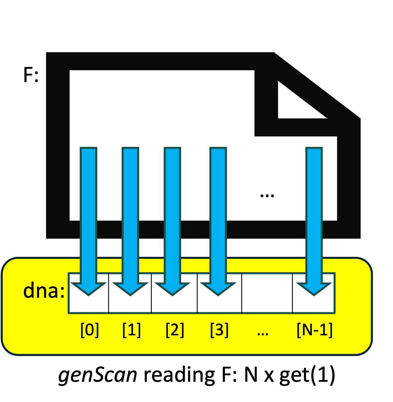
Suppose the genome file contains N characters. Then in our original version, the readFile() function calls istream::get() and string::operator+=() N times, and both of these are time-consuming. We might visualize that version of readFile() as shown on the right:

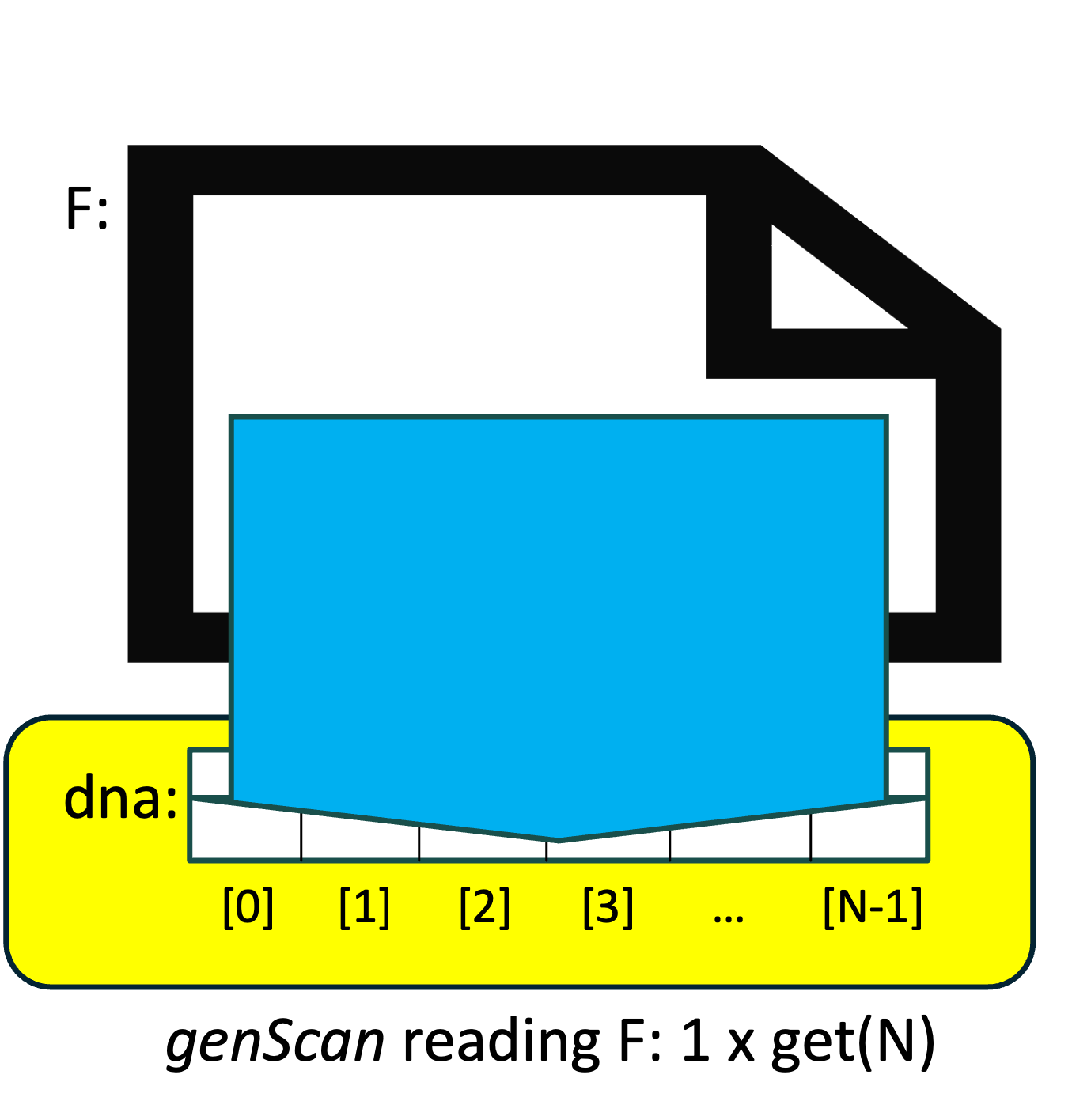
By contrast, our revised version of readFile() first calculates N, the number of characters in the file, uses that value to resize our string& parameter seq (which is an alias for our main() function's dna variable), and then calls istream::get() once, but tells it to read N characters instead of just a single character. We might visualize this as shown on the left:

By (i) resizing the string ahead of time instead of relying on string::operator+=() to "grow" the string when necessary, and (ii) replacing N calls to get(1) with a single call to get(N), our revised version of readFile() accomplishes the same task, but does so far more efficiently.

Before we proceed any further, let's save a copy of this version:

   cp genScan.cpp genScan_v2b.cpp

At this point, we have done about as much as we can using a traditional (i.e., sequential) software design. We have significantly improved the performance of genScan, but despite our changes, it still takes several seconds. To solve this problem any faster, we need a completely different approach. Thankfully, modern hardware makes this possible!

Part II. Parallel Computing

The versions of genScan we have written so far do not take advantage of today's hardware capabilities. In this section, we will see one way we can do so.

Moore's 'law'

Moore's 'law' was a 1965 observation by Intel co-founder Gordon Moore that the number of transistors that fit on a computer chip was doubling every two years. This remarkable doubling phenomenon held through at least 2020, and it allowed manufacturers to build a new generation of computers every two years that were twice as powerful as the previous generation.

Multicore CPUs

Transistors are used to build (among other things) the core logic of a computer's central processing unit (CPU)--the hardware that actually performs a computer program's instructions. Before 2005, Moore's 'law' let CPU manufacturers pack more and more functionality into their CPUs, so every two years, the CPUs were twice as capable as they had been previously.

By 2005, transistors had shrunk so much that all of the core logic of a very powerful processor could fit into just half of the space of a standard CPU chip. This created a dilemma for the manufacturers: What should they do with the rest of the space?

The answer was the 2006 dual-core CPU--a CPU that, in essence, had two CPUs-worth of core logic within a single CPU chip. Unlike previous CPUs, dual-core CPUs could literally do two things at once, since the first core could be performing one instruction at the same time as the second core was performing a different instruction. By 2008, two cores took up just half of the space in the chip, so the manufacturers created quad-core CPUs--chips that could perform four different instructions simultaneously.

This progression has continued; if you are willing to pay the asking price, today's manufacturers will happily sell you a CPU with 64 (or more) cores:

In Linux, you can find the number of physical cores available on your system by entering this in your Terminal:

   lscpu | grep "Core(s)"

A different Linux command reports the number of "processing units" on your system:

   nproc

Multithreading

CPUs and cores are hardware; this exercise is about writing faster software. The smallest software unit that can run independently on a CPU core is called a thread.

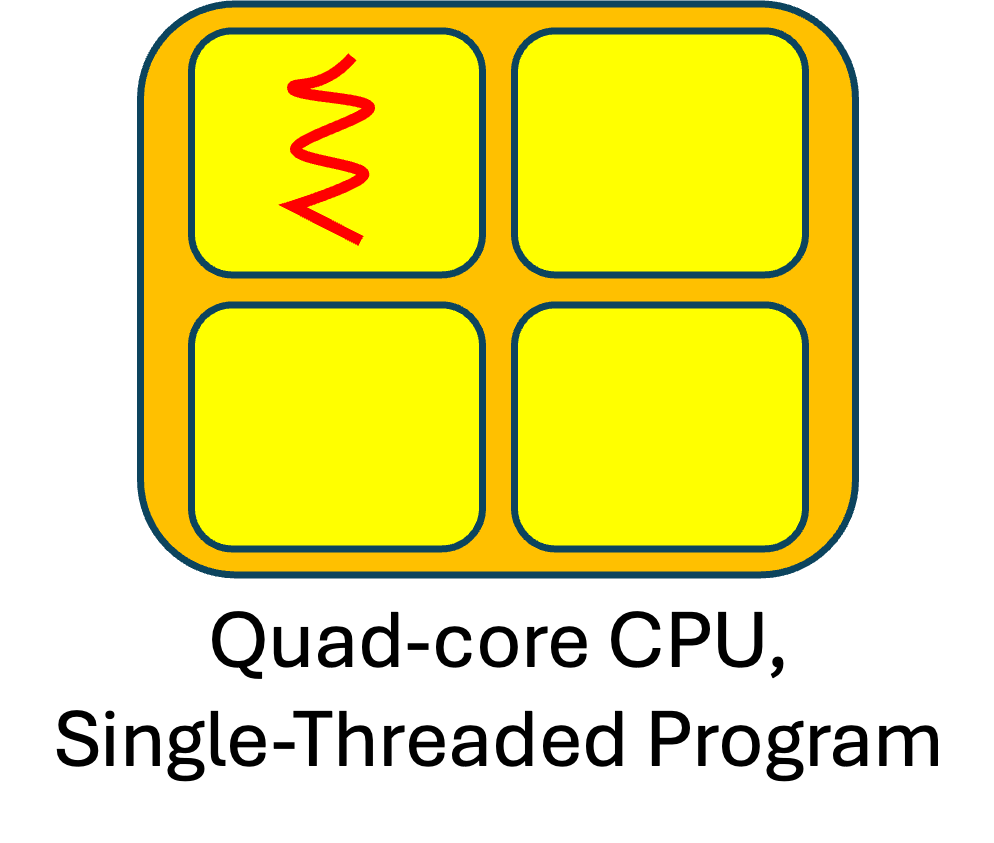
Prior to 2006, CPUs just had a single core, and since a single core could only perform one statement at a time, traditional programs had (and continue to have) just one thread. What happens when we run such programs on a multicore CPU? That program's single thread uses just one of the cores. The versions of genScan we have written so far have all been traditional, single-threaded programs.

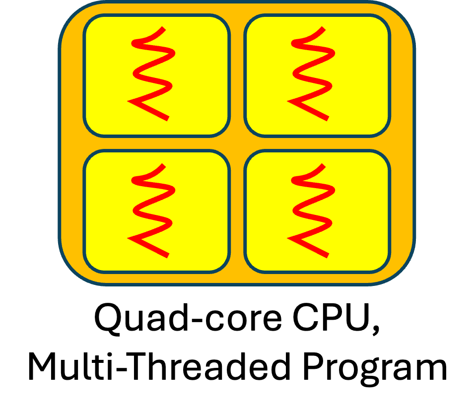
To illustrate, if we have a quad-core CPU and we use a red "squiggly line" to represent a thread, we might visualize the executions of each of our previous versions of genScan as shown to the right:

On a quad-core CPU, a traditional (single-threaded) program uses just 25% of the CPU's potential; on an 8-core CPU, it uses just 12.5%; on a 16-core CPU, it uses just 6.25%; and so on. The more cores a CPU has, the more potential performance a traditional program wastes.

The versions of genScan we have written so far have all used just a fraction of computer's hardware capabilities. How can we revise genScan to use all of its potential?

A program that solves its problem using multiple threads is called (surprise!) a multithreaded program. How do we write such a program?

The first step is to redesign our algorithm to use multiple threads instead of just one.

Divide-And-Conquer, Parallel Style

There is an old saying:

"Many hands make light work."

One way to do this is to have our program spawn additional threads, have each thread read a different chunk of the genome file, count the number of occurrences of the subsequence in its chunk, and then sum those partial counts to get a total count.

Let's visualize this using four threads: thread₀, thread₁, thread₂, and thread₃. We first have the four threads divide the input file F into four chunks that are as equal in size as possible. We also want each thread_i to have its own data structure dna_i, whose size is the size of its chunk:

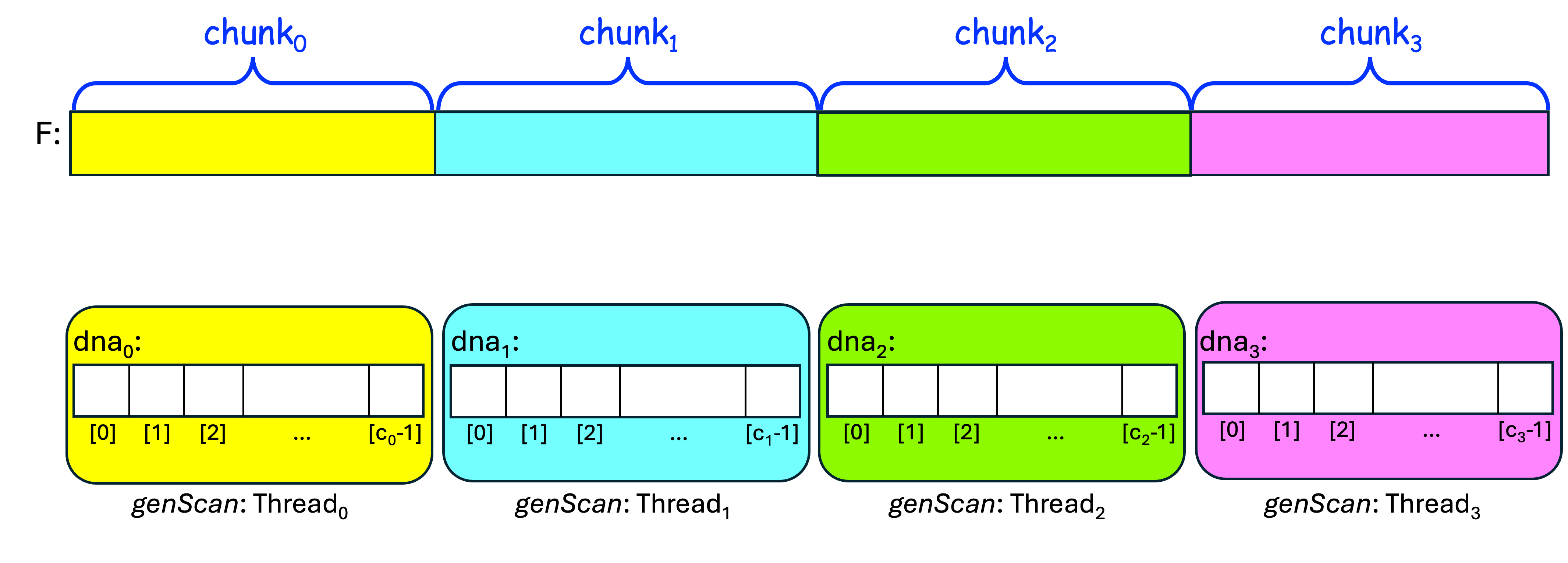
After doing that, we want each thread_i to read its chunk_i from F into dna_i, using the one-read approach:

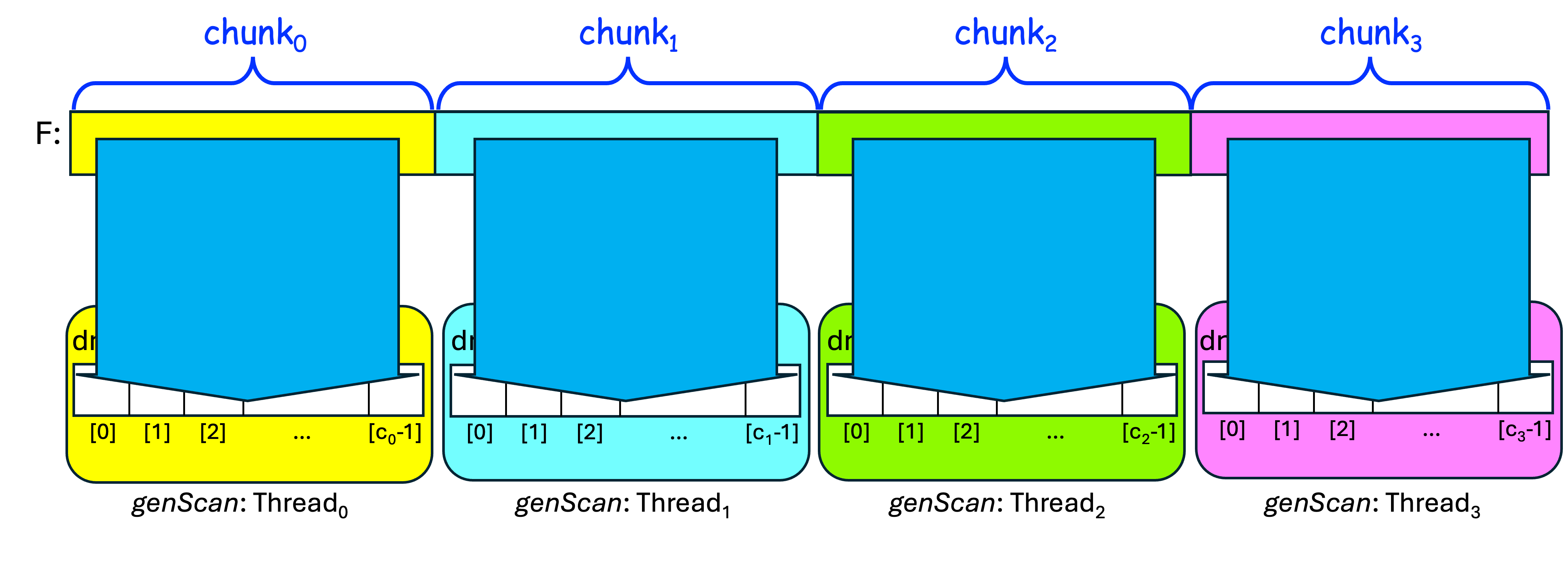
Once it has its chunk_i in dna_i, each thread_i can then scan its dna_i for the subsequence, and store the results in count_i. We then have to sum these partial count_i values into a total count.

If the threads perform these steps simultaneously (i.e., in parallel), this approach should give us faster performance. (This is simplified; we must also account for subsequences that cross the boundaries between two chunks--we'll see how to do that shortly--but for now, this should give you the basic idea.)

Let's organize these ideas into an algorithm for our problem.

A Parallel Algorithm

We have seen how to get the file name F and the subsequence subSeq from the user, so let's assume we've already done those steps. The table below presents our original algorithm and a new parallel algorithm, for easy comparison:

Steps 1 and 2 of our new parallel algorithm are obviously more complicated than steps 1 and 2 of our original algorithm. In the rest of this exercise, we'll see one way we can implement this new algorithm.

Implementing Our Algorithm in OpenMP

OpenMP is a library created to add multithreading capabilities to C/C++ and other inherently sequential languages. It makes it relatively easy to "parallelize" an already-existing sequential program, so we will use it to implement our algorithm.

The table below shows the main() function of our original algorithm beside a main() function that implements our parallel algorithm using OpenMP:

int main(int argc, char** argv) { 
  string fileName;
  string subSeq;
  string dna;

  double startTotalTime = omp_get_wtime();
  processCommandLineArgs(argc, argv, fileName, subSeq);

  double startReadTime = omp_get_wtime();
  readFile(fileName, dna);
  double readTime = omp_get_wtime() - startReadTime;

  double startScanTime = omp_get_wtime();
  long count = scan(dna, subSeq);
  double scanTime = omp_get_wtime() - startScanTime;

  double totalTime = omp_get_wtime() - startTotalTime;

  printResults(subSeq, count, 
                readTime, scanTime, totalTime);
}

int main(int argc, char** argv) { 
  string fileName;
  string subSeq;

  double startTotalTime = omp_get_wtime();
  processCommandLineArgs(argc, argv, fileName, subSeq);

  long count = 0;
  int P = 0;
  double readTime = 0.0, scanTime = 0.0;

  #pragma omp parallel reduction(+:count)
  {
    P = omp_get_num_threads();
    int id = omp_get_thread_num();

    double startReadTime = omp_get_wtime();
    ParallelReader<char> pReader(fileName, MPI_CHAR, id, P);
    vector<char> dnaChunk = pReader.readChunkPlus(subSeq.size()-1);
    pReader.close();
    #pragma omp master
    readTime = omp_get_wtime() - startReadTime;

    double startScanTime = omp_get_wtime();
    count = scan(dnaChunk, subSeq);
    #pragma omp master
    scanTime = omp_get_wtime() - startScanTime;
  }

  double totalTime = omp_get_wtime() - startTotalTime;

  printResults(P, subSeq, count, 
                 readTime, scanTime, totalTime);
}

01
02
03
04
05
06
07
08
09
10
11
12
13
14
15
16
17
18
19
20
21
22
23
24
25
26
27
28
29
30
31
32
33
34

Take a few moments to replace the body of genScan's main() function with this new definition and save your changes.

For the casual reader, here is a quick overview of how our revised main() function works:

1. The OpenMP directive #pragma omp parallel on line 12 spawns P-1 new threads for a total of P, implementing step 0 of our algorithm. We'll see how to specify P shortly.
2. The curley-braces ({ and }) on lines 13 and 28 and the statements between them comprise a C/C++ block statement, which all P threads will perform. The statements within this block statement (lines 14-27) perform steps 2 and 3 of our algorithm.
3. Lines 14 and 15 call OpenMP functions that let each thread compute the number of threads (P), and the id number of this thread (i for thread_i) -- values that are needed to divide the work among the threads. Each thread will get the same value for P, but its own unique id value. In the original thread id will equal 0; the other threads will get id values from 1 through P-1.
4. Lines 18-20 construct a ParallelReader object and use its readChunkPlus() method to perform step 1 of our algorithm.
5. Line 25 performs step 2a of our algorithm.
6. Back on line 12, the reduction(+:count) clause performs step 2b of our algorithm, but only when all threads have finished and execution leaves the C/C++ block statement (line 28).

Adjusting scan()

Since a ParallelReader may be used to read a file containing numbers, the ParallelReader::readChunkPlus() method returns a vector instead of a string. Since our existing scan() function is expecting a string, we must revise scan() in order for genScan to build without errors.

The table below shows our previous version (v2a) alongside a revised version that employs almost the same logic, but replacing our string paramater seq with a vector parameter chunk.

long scan(const string& seq, const string& subSeq) {
  long skip = subSeq.size();
  long count = 0;

  size_t pos = seq.find(subSeq, 0);
  while (pos != string::npos) {
    ++count; 
    pos = seq.find(subSeq, pos+skip);
  } 

  return count;
}

long scan(const vector<char>& chunk, const string& subSeq) {
  long skip = subSeq.size();
  long count = 0;

  vector<char>::const_iterator 
       it = search(chunk.begin(), chunk.end(), 
                    subSeq.begin(), subSeq.end());
  while (it != chunk.end()) {
    ++count;
    it = search(it+skip, chunk.end(),
                 subSeq.begin(), subSeq.end());
  }

  return count;
}

Take a moment to replace the body of scan() with this new definition and save your changes.

Note that this new definition replaces find() with search(). The find() in v2a is a string method that searches a string for a substring. While vector has a find() method, it does not allow us to search the vector for a substring, because unlike a string, a vector may contain non-character items.

But vector is a container from the C++ standard template library (STL), which also contains algorithms. These include the STL search() algorithm, which can be used to search a vector<char> for a char sequence. When successful, search() returns an iterator to what you are seeking; otherwise, it returns its second argument, so the definition above uses this to control the while loop.

Adjusting printResults()

You will also need to alter printResults() to have it display the number of threads used. Do this so that when run with P=2 threads, its output will begin with:

2 threads found ... 

3 threads found ... 

This adjustment is straightforward, so we leave it to you. If you experience difficulty, consult your neighbor and/or your instructor.

Building genScan

If we try to build genScan at this point, we will still get errors and warnings (feel free to try!). We need to adjust two more things before it will build for us:

1. The STL search() algorithm is declared in a standard C++ header file named algorithm, and ParallelReader is defined in OO_MPI_IO.h, which you should have downloaded when you began this exercise. We need to #include those files, so near the beginning of genScan.cpp, find and uncomment the lines

      #include <algorithm>
      #include "OO_MPI_IO.h"

   Then save your changes.
2. OO_MPI_IO.h uses a parallel library called MPI, which stands for the Message Passing Interface. MPI code can be built with the g++ compiler, but doing so requires several additional compiler flags. Rather than make us supply all of those flags, MPI provides a 'wrapper' named mpicxx that calls g++ with the needed flags. The takeaway is that we want to build genScan using mpicxx instead of g++.

   To accomplish this, use any text editor to open the Makefile and find the line:

      CC = g++

   and change it so that it instead reads:

      CC = mpicxx

In your Terminal, you should now be able to build genScan by entering:

   make

Running genScan

Since genScan is now using OpenMP multithreading, we need to adjust how we invoke it. To run it using P threads, you would enter:

   OMP_NUM_THREADS=P ./genScan /tmp/Felis_catus_9.dna.plain CAT

   OMP_NUM_THREADS=7 ./genScan /tmp/Felis_catus_9.dna.plain CAT

Data Collection and Visualization

To gauge how well genScan works, we want to run it with increasing values for P (e.g., 2, 4, 6, ...), to see how its times change as P increases.

Measuring time can be a "noisy" operation, and as the time-values get small, there may be significant fluxuations in the times omp_get_wtime() reports.

To minimize the effects of such fluxuations, we will run genScan three times for each value of P. Since each run generates three time-values (read, scan, total), these three runs--called trials--will generate a total of nine time-values for each value of P. We will enter these nine time-values in our spreadsheet, and it will calculate their minimum time-values for us.

In your copy of the spreadsheet, scroll down and click the Parallel tab at the bottom to expose a second sheet. Take a moment to look over this new sheet to get a feel for how it is organized.

For each value of P in column A (2-12), you can run 3 trials, report their Read/Scan/Total times in columns B-J, and the rest of the sheet should update correctly. In particular, the Min Times in columns K-M should update automatically as you enter your trial-times. The stacked-column chart at the bottom uses these Min Times.

Note that the trial-times for P=1 (row 4) are blacked out; the Min Times in that row should already contain the values you reported for genScan version v2b on your spreadsheet's Sequential tab.

Note also that you should only change the values in cells B5 through J10. If you try to change any of the other already-defined cells, the spreadsheet will warn you that you are not supposed to be changing those cells.

If you have not already done so, arrange your Terminal and spreadsheet so that they are side-by-side (i.e., adjust their positions and if necessary, their sizes) so that the output from genScan and your spreadsheet's cells are both visible. Being able to see both at once should speed up the rest of this exercise for you.

In your Terminal, run genScan with P=2:

   OMP_NUM_THREADS=2 ./genScan /tmp/Felis_catus_9.dna.plain CAT

Linux Time-Saving Tip: Assuming you have a scroll-wheel mouse:

1. In your Terminal, highlight / select the three time-values (i.e., left-click+drag over all three time-values) but do not copy them,
2. In your spreadsheet, point your mouse-cursor at cell B5 (i.e., where you want to paste), and
3. middle-click (i.e., click your mouse's scroll-wheel).

(If this is not working for you, make certain you are running genScan from the commandline within an actual Terminal, not from within an integrated desktop environment (IDE) that replaces tabs with spaces.)

That finishes Trial 1 for P=2, so let's return to the Terminal for Trial 2, P=2.

Using your keyboard's up-arrow, use the same command as before to re-run genScan.

When it finishes, use the same Linux Time-Saving Tip as before to highlight+paste the three new time-values into your spreadsheet beneath Read/Scan/Total for Trial 2, P=2.

Repeat this procedure again to generate new time-values for Trial 3, P=2 and paste these new times into your spreadsheet under Trial 3, P=2.

After you do this, the values for P=2 under Min Trial Times should automatically reflect the minimum values from your three trials, and if you scroll down to this sheet's chart, the stacked-column above P=2 should reflect those minimum values.

Next, let's use this same approach for the three trials for P=4.

Linux Terminal Tip: In your Terminal, use your keyboard's up-arrow to retrieve the previous command. Then use your left-arrow to back the cursor to the space after OMP_NUM_THREADS=2, use backspace to erase the 2, press 4 to replace that 2, and then press Enter (or Return) to run genScan with P=4.

When genScan finishes, use the highlight+paste shortcut to transfer its three new times from your Terminal to your spreadsheet, on the P=4 row beneath the Trial 1 Read/Scan/Total columns.

Repeat this process twice more to generate the Trial 2 and Trial 3 times for P=4. Then look at the chart to verify that the stacked-column above P=4 reflects the minimum times from these trials.

Now that you've completed the three trials for P=2 and P=4, repeat this 3-trial procedure for the remaining values of P (6, 8, 10, 12) before continuing...

Congratulations--you have used parallel computing and multithreading to speed up the solution to a real-world 'big data' problem!

Optional: Answer an Alternative Research Question

Suppose a group of housecat-researchers are playing the "Catan" board game, and one of them muses:

I wonder how many times the subsequence 'CATAN' appears in our genome?

Using what you have learned in this exercise, answer this question.

Before You Go

Now that you have finished the exercise, please help us gauge its effectiveness by completing this very short survey.

Thank you for your help--we hope you've enjoyed this exercise!