The purpose of this assignment is to practice:
- using turtle method calls
- computing mathematical expressions
- using
ifstatements.
You’ll also be getting a preview of what we’ll learn about next week–loops!
Introduction 
One can use a Monte Carlo technique to estimate the value of pi, by
simulating randomly throwing darts at a big square piece of wood, and
calculating how many land within a circle drawn on the wood. We can use
the same technique for estimating the area under a curve, where the
function creating the curve cannot be integrated in the normal way. The
Gaussian integral is just such an integral. The Gaussian function,
$e^{-x^2}$ (that is, e to the -x squared), produces the following
graph:
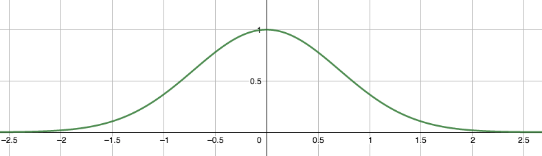
Fancy integration techniques show that the area under this curve is $\sqrt{\pi}$.
Our estimates should produce a number close to that.
In this assignment, you will create a canvas and randomly place dots on it, counting the total number of dots placed and the number of dots that fall below the line.
Step 1: Create program file 
Download template-turtle.py and rename it integration.py in an
appropriate folder.
Update the header documentation as usual.
Step 2: Draw the coordinate axes 
We want to be able to graph the Gaussian function from -3 to 3 in the x (horizontal) direction and from 0 to 1.5 in the y (vertical) direction.
If we were using the default coordinate system, the entire plot would be extremely small. Fortunately, the turtle module gives us a convenient way to zoom in.
So:
- Use the
window.setworldcoordinates()function to set the lower-left and upper-right corners of the canvas. - Draw the x and y axes lines in the window. (Don’t worry about axis labels or gridlines.) You may want to use
pen.setpositionandpen.setheadingto move the turtle pen to where you want it. - Run your code to make sure everything looks correct.
Step 3: Plot the true Gaussian function values 
On the graph you just drew, plot the Gaussian function in black with x
values ranging from -3 to 3. Note that you will want to plot more points
than just the integer values for x. For this assignment, 1000 data
points should be plenty. Use this for loop:
for i in range(1000):
    # your code goes here.
The first code in the loop needs to transform i from the values 0, 1,
2, …, 999 to x values that range from -3.0 to 3.0 To map i to x,
use the following code:
x = -3.0 + (i / 1000) * 6.0
This will give 1000 x points varying from -3.0 to 3.0. At each
x value, compute the corresponding y value by using the gaussian
function and move the pen to the next point. This will plot the function
using a sequence of short lines. To compute the y values, you’ll need
to use the
math.exp()
function.
Hint on speed: Once you get this part running, you might want to call pen.speed("fastest") before it to speed up the turtle.
If you still want it faster, try adding window.tracer(10) (or 100 or 1000).
Step 4: Throw darts 
Now, you need to write code to simulate randomly throwing darts at the board, and counting how many land below the line.
We want to throw 50 “darts” at this “dartboard,” so create a constant
called NUM_DARTS and initialize it to 50. (Notice that there is a section in the template for constant definitions.) Then, write a for loop, just
like above, to iterate NUM_DARTS times:
n_darts_below_curve = 0
for dart in range(NUM_DARTS):
    # your code goes here
Inside the loop, get random values for x and y using
random.uniform().
You want to get random values for x between -3 and 3, for y between 0 and 1.5.
Write a line of code to print out the values of x and y to observe the
values and then run your code to make sure things look good. Remove
these print statements once things appear to be running correctly.
Next write an if statement to determine if the y value for that x value
is on or below the Gaussian function or not. If it is, place a dot,
drawn in red at (x, y); otherwise plot it in blue.
Consult the Python Turtle documentation to find out more about the dot()
method.
Also, if the dart is below the line, increment n_darts_below_curve (by using n_darts_below_curve = n_darts_below_curve + 1) to keep track
of this. You’ll need to initialize this counter to 0 at the beginning of
the loop, as the example above does.
Step 5: Compute the estimate 
Now, compute your estimate of the area under the curve. First, compute the total area of the plot area. Then, compute what fraction of the dots ended up on or under the curve. (Use your counter.)
Assuming uniformly distributed “darts,” the area under the curve can be estimated by the ratio of darts on or under the curve divided by the total number of darts multiplied by the entire area of the plot.
At the end of the code, print out the computed value for the area under
the curve, and your estimate for the value of $\pi$ (you will need to square the
area under the curve to get $\pi$).
Remember to use good variable names.
Run this a few times. Is your estimate of pi at all close? What could you do to make it better?
Step 6: Improve the estimate 
With 50 darts, your estimate of $\pi$ will probably not be very accurate. So, increase the number of darts!
Set NUM_DARTS to 5000 and rerun your code.
Hints about speed: 5000 points will take some time, so somewhere before the darts loop:
- Use the
hideturtle()method on your turtle to hide the turtle - Use
window.tracer(1000)to reduce the screen update rate to speed up processing. - Note that it is not necessary to pick the pen up and down when using
dot().
Step 7: Submit your code and a screen shot 
First, make sure the documentation header includes:
- Your name and userid
- The assignment number and a brief description of what the code does.
Submit on Moodle (not ZyBooks this time!):
- Your code
- A screenshot of your completed simulation run 5,000 times. Name the file
screenshot.png.
Grading Rubric 
10 points total:
-
60%: correctness and completeness
-
30%: understandability:
- blank lines and comments before sections of code
- spacing around expressions
- header with all required information
- no extraneous code or variables
-
10%: the screenshot