Lab 11: Multidimensional Arrays and Vectors

Introduction

We have seen that we can use arrays or vectors to store sequences of values. For example, the declarations

    double arrvec[50];

and

    vector<double> arrvec(50);

define an object arrvec as a container that can store 50 double values.

We usually visualize such a container as one-dimensional objects — i.e., a linear sequence of values. And as we saw in the previous lab exercise, a single index is sufficient to access the elements of a one-dimensional array or vector because it is a linear structure.

There are, however, many objects that are more naturally visualized as having two (or more) dimensions such as a tic-tac-toe game

and a magic square

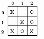
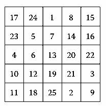
which are organized into rows and columns.

Such two-dimensional structures can be represented in a program as an array of arrays such as

    int magicSquare[3][3];

or as a vector of vectors:

    vector< vector<int> > magicSquare;

To access an element of a two-dimensional array or vector, two indices are needed: the first to specify the row in which it located and the second to specify a column within that row. For example, we could access the integer 17 in the upper left corner of magicSquare with the expression

magicSquare[0][0]

the integer 11 in the lower left corner with

magicSquare[4][0]

and the integer 13 in the center with

magicSquare[2][2]

In this lab exercise, we will use a two-dimensional array to implement an interesting game known as the game of life.

The Game of Life

The Game of Life (also known simply as Life) is a cellular automaton that was devised by the British mathematician John Conway as a simple model of a society of organisms. The "playing board" is a rectangular grid of cells. Each cell in the grid (except along the border) has eight neighboring cells: 3 cells above it, 3 cells below it, and 1 on each side of it.

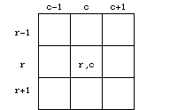
Each cell may have an organism in it that we'll represent by an asterisk, *.

The game consists of a series of generations. You provide the initial configuration of organisms, and each generation thereafter is determined by applying the following rules to the previous generation:

If an empty cell has exactly three neighboring organisms, then an organism is born in that cell.
If a cell has fewer than two neighboring organisms, then an organism in that cell dies of loneliness.
If a cell has more than three neighboring organisms, then an organism in that cell dies of overcrowding.

For example, suppose that we begin with the following configuration of three organisms:

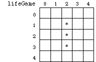
Then applying the rules, we can generate the next generation:

Cells in the first column — locations [0][0], [1][0], [2][0], [3][0], [4][0] — and those in the last column — [0][4], [1][4], [2][4], [3][4], [4][4] — have no neighbors and thus remain empty.
Cells [0][1], [1][1], [0][2], [0][3], [1][3], [3][1], [3][3], [4][1], [4][2], and [4][3] each have one neighbor so they also remain empty.
Cells [1][2], and [3][2] each have one neighboring organism, so the organism in them dies of loneliness.
Cells [2][1], and [2][3] have three neighboring organisms, so an organism is born in each of them.
Cell [2][2] has two neighbors, so it remains unchanged.

Represented graphically, the second generation is

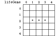
To get the third generation, we apply the rules to the second generation. Organisms are born in cells [1][2] and [3][2] and the organisms in cells [2][1] and [2][3] die, which means that we have returned to the original configuration!

This particular configuration continues to oscillate back and forth from generation to generation. We might think of this as representing a society of organisms that although changing from one generation to the next, it remains stable if it is not disturbed by outside influences.

Other configurations grow larger and larger with each generation until the entire grid is nearly filled —a population boom. Others grow smaller and smaller until all organisms are dead, modeling societies that eventually become extinct. Examples of these kinds of behavior will be described later in this lab exercise.

Files

life.cpp implements the game of Life. It reads the initial configuration from a data file, stores it in a two-dimensional array, and displays its contents so it can be checked by the user. It will then ask the user for the number of successive generations to be produced and will then produce and output them to a file specified by the user.
You should download this file and add your name and other information required by your instructor to the opening documentation. As you work through this lab exercise, you will be adding to and/or modifying this program.

The data files to be read by this program begin with the number of rows and columns in the grid followed by rows of 0s and 1s, one for each row in the grid, and each row containing an entry for each column in the grid — 0 representing an empty cell and 1 representing a cell occupied by an organism. For example, the file test.life that you will use in this lab exercise contains the following initial configuration for the simple three-organism oscillating pattern described earlier:
5 5 0 0 0 0 0 0 0 1 0 0 0 0 1 0 0 0 0 1 0 0 0 0 0 0 0
Here are other data files you should try with your program after you get it written: stable.life, quick.life, cross1.life, cross2.life, glider.life, gliders.life, and blank.life.

Design

This lab exercise is to complete the life.cpp program. This will involve adding and testing code to do the following:

Read the grid configuration from a data file and store it in a two-dimensional array.
Display the contents of this file on the screen so they can be checked.
Write a display() function to output each generation to a file via an ostream.
Write a generate() function to generate the next generation.

Implementation

Now that we have the operations identified, we can start writing code to implement them. So open the file life.cpp which contains a partially-written program that you will be completing and testing in this lab exercise.

Modeling the Life grid

To represent the grid we will use a two-dimensional array (or if your instructor prefers, a vector of vectors.) However, to create this array, we need to know:

— its dimensions, and
— the type of its elements.

We can define a two-dimensional array type with a declaration of the form

typedef ElementType ArrayTypeIdentifier[ROWS][COLUMNS];

where ROWS and COLUMNS are integer constants that specify the array's dimensions;
ElementType is the type of its elements; and
ArrayTypeIdentifer is the name of this new type that we have defined.

Question #11.1 Define an array type named LifeGrid at comment #1 near the beginning of life.cpp. For this exercise, all of the grids will have 50 or fewer rows and columns so you can use this to specify the number of rows and columns. As explained next, we will use short (or short int) for the type of the array elements.

We turn now to the question of why we are using short for the type of the cells when all of our examples represented the presence of an organism with an asterisk (*) and an empty cell with a blank. So wny not use char for the cell type?

If we look at the most important operation of a LifeGrid object — generating a new generation — and at the rules for producing a new generation, we see that they involve counting neighboring organisms. This would mean counting the number of times a certain character — an asterisk — appears in each of the neighboring cells by comparing each of their contents with an asterisk. And this must be done for every cell in the grid! But if we use a grid of integers rather than characters, representing the presence of an organism with 1 and an empty cell by 0, no comparisons are required — just sum the values in the neighboring cells! And because there are only eight neighbors, we can use short integers to reduce the memory requirements for this array.

But what about the earlier pictures of a LifeGrid object? If the asterisks are replaced by 1s and the empty cells with 0s, it surely won't be as picturesque as the asterisk-blank representation! The solution? Let's use the 0-1 representation in the data file that will be input and stored internally as a grid of 0s and 1s but then output it as the more visually pleasing grid of asterisks and blanks!

Constructing the `LifeGrid`

After the opening information about the game of Life and the maximum size allowed for a grid, the main() function in life.cpp begins by creating the LifeGrid array grid as a MAX_ROWS x MAX_COLUMNS array. It then asks the user for the name of a file containing a Life pattern and vvvopens an ifstream named fin to that file.

For simplicity, we will assume that the first line of the file contains two integers, the number of rows and the number of columns in the grid of cells. The remainder of the file will then be a grid of starting values for those cells. For example, our test.life input file provides the starting configuration for the three organism oscillating pattern:

In this 5 × 5 grid (as specified in the first line of the file), each 1 represents a cell containing an organism and each 0 represents a cell without an organism. Note: Any whitespace can be used to separate the cells in the file; in this example, single spaces and newlines were used to make it easy to read.

Question #11.2 At comment #2 in main() of life.cpp, write code to read the number of rows and columns in the grid of cells from the data file via the input file stream fin. Then use nested for loops to copy the 0s and 1s from the data file via the ifstream fin into the upper-left corner of grid — i.e., this grid of cells would be copied into rows 0, 1, ..., 4 and columns 0, 1, ..., 4 of grid.

Now that the Life configuration has been transferred from the file to grid, we can move on to task #2 in our design plan:

2. Display the contents of this file on the screen so they can be checked.

Question #11.3 At comment #3 in main() of life.cpp, display the contents of grid using the same format as shown above:
5 5 0 0 0 0 0 0 0 1 0 0 0 0 1 0 0 0 0 1 0 0 0 0 0 0 0

The `display()` Function

The format of our output of grid is the same as that in the data file from which its contents were transferred. But in the game of Life, the grids are shown as grids of cells in which an asterisk is used instead of 1 and a space instead of a zero. The function display() will output grid in this asterisk-space format. And to give it somewhat of a grid-like appearance, it will output periods to mark the corners of the cells.

Also, for some patterns it can take a large number of generations to study their behaviors. To make it easier to study the successive generations, we will output them to a file so they can be examined later.

Question #11.4 The opening statements of the function display() output a top border for the grid by writing a series of period-space combinations ( ". " ) to a file via the ifstream fout. At comment #4 in the definition of this function, write nested loops to output the rest of the grid by outputting in each row:
". " (to mark the left border) followed by "* " for each 1 and ". " for each 0 in that row.
For the file "test.file", the first two generations will be output as:
Generation #1 . . . . . . . . . . . . . . . . . . . . . . . * * * . . . . . . . . . . . . . . . . . . . . . . . Generation #2 . . . . . . . . . . . . . . . . . * . . . . . . * . . . . . . * . . . . . . . . . . . . . . . . .

Here is an algorithm for this part of display() that may help with writing the code:

For each index r in the range 0 .. numRows do the following:

Output ". " // for the left border
For each index c in the range 0 .. numColumns do the following:
If grid[r][c] is 1
Display "* "
Otherwise
Display ". "
Move to a new line.

Generating The Next Generation

The function generate() is the workhorse of this program because it must encode the rules of the game:

For each cell c in the grid:

If c has exactly three neighboring cells containing 1s, then
c should contain a 1.
Otherwise if c has fewer than two neighbors containing 1s
or c has more than three neighbors containing 1s, then
c should contain a 0.

In order to process all of the cells, we will need two nested for loops again to process the rows and columns of grid. The inner loop should count the number of neighbors for the current cell and then set the value of that cell appropriately as required by the rules of the game.

But there are two problems. First, the next generation is determined by the current generation. We cannot overwrite the current generation with the next one because the current generation is needed to determine the next. So we will begin by making a copy of grid and then use this copy to calculate each cell's neighbors.

The second problem is that cells at the edges of the grid do not have the required eight neighbors. To simplify things, we'll assume that these are "boundary" cells and don't ever change; so we can simply exclude them from consideration by letting the row index run from 1 to numRows − 1 and the column index run from 1 to numColumns − 1.

This gives the following (partial) algorithm for generating the next grid of cells:

Make a copy newgrid of grid.
For each index r in the range from 1 to numRows − 1
For each index c in the range from 1 to numColumns − 1
a. Calculate topNeighbors = grid[r - 1][c - 1] + grid[r - 1][c] + grid[r - 1][c + 1]
b. bottomNeighbors = ???
c. sideNeighbors = ???
d. Calculate neighbors = sum of the three preceding sets of neighbors.
e. Apply the rules of the game to set newgrid[r][c]
Now copy newGrid to grid. (Because it is a reference parameter, it will be passed back to main().)

As we noted earlier, because each cell is an integer — 0 representing an empty cell and 1 representing an organism — we can simply add the values in the surrounding cells to compute the number of neighbors in Step 2-d of the algorithm.

The algorithm, however, leaves two of the computations unfinished for you to complete. Use the topNeighbors computation and the picture of a cell at the beginning of this exercise to finish the other computations.

Question #11.5
Complete the algorithm above for generating a new Life generation by finding the formulas to replace the ???s in the computations of bottomNeighbors and sideNeighbors.

Then, using this algorithm, complete the definition of the function generate(). Compile your code, and test the program using test.life. When completed, your program should be ready to process other initial configurations.

Playing the Game of Life

Playing the game of Life consists of creating initial configurations of organisms, and then running the program and stepping through the generations to see what happens to the society as time passes. Although test.life gave us a simple way to check how our program was working, it is a rather uninteresting configuration because very little changes as time passes.

Now try the configuration in stable.life. Here the generations don't change at all from one to the next — thus the name. Some initial configurations appear to be unstable but after awhile, they reach stability. Try quick.life for an example. And for some configurations, The society of organisms quickly breaks down and after a few generations, becomes extinct; cross1.life is one such example.

Sometimes adding or removing a few individuals makes all the difference between on how a society changes. To illustrate thus, here is the initial configuration in cross1.life; it is sometimes referred to as an iron cross:

 

    * * *
      *
*     *     *
* * *   * * *
*     *     *
      *
    * * *

Now suppose we add an organism at the end of each cross, as in cross2.life:

 
        *
      * * *
        *
  *     *     *
* * * *   * * * *
  *     *     *
        *
      * * *
        *

Question #11.6: How do the generations of this cross-society compare with those of the first cross-society?

Each of our configurations has thus far been symmetric, but there is no requirement that this be the case. Some asymmetric configurations are more interesting than the symmetric ones. For example, try glider.life. This society goes through a periodic cycle of four configurations, and each cycle moves a space across the grid. The result is a migratory society that moves through the grid as time passes. This behavior is similar to that of some insect colonies or flocks of birds.

When two gliders collide, the results are unpredictable. Sometimes they lead to extinction of both societies and sometimes they result in something entirely different.

Question #11.7: What happens with the gliders in gliders.life? Try at least 35 generations. (Looks like we've come full circle!)

Experiment

The file blank.life contains a 25 × 35 grid of all 0s. Make several copies of this file and edit them to create your own original configurations and run them through the Life program. See if you can find a simple initial configuration that is still changing after 100 generations.

Lab Home Page

Report errors to Larry Nyhoff (nyhl@cs.calvin.edu)