flowchart LR
    A1[("Training Data (X and y)")] --> B{{fit}}
    A2[Model Object] --> B
    B --> FM[Fitted Model]
    FM --> C{{Predict}}
    B2[(New data X)] --> C
    C --> D[("predicted y's")]
Learning Machines
Ken Arnold
Intro Activity: Teachable Machine
Team up with one or two other people near you.
- Go to https://teachablemachine.withgoogle.com/train/image
- Train a simple classifier using your webcam. Don’t worry about making it super accurate. Ideas: which hand are you holding up? happy or sad face? looking left or right? two colors?
- Discuss with your partners how you might quantify the performance of your classifier. Evaluate your classifier according to your plan.
- On a nearby whiteboard, write (1) your classifier’s task and (2) your evaluation results.
Discuss with your partners:
- What were the inputs and outputs of this system? Where did its training data come from? How did it know what it should learn?
- What did the evaluation number tell you about the system? What did it not tell you?
- True or False: the model continuously learned from its mistakes.
- Is “Teachable Machine” intelligent?
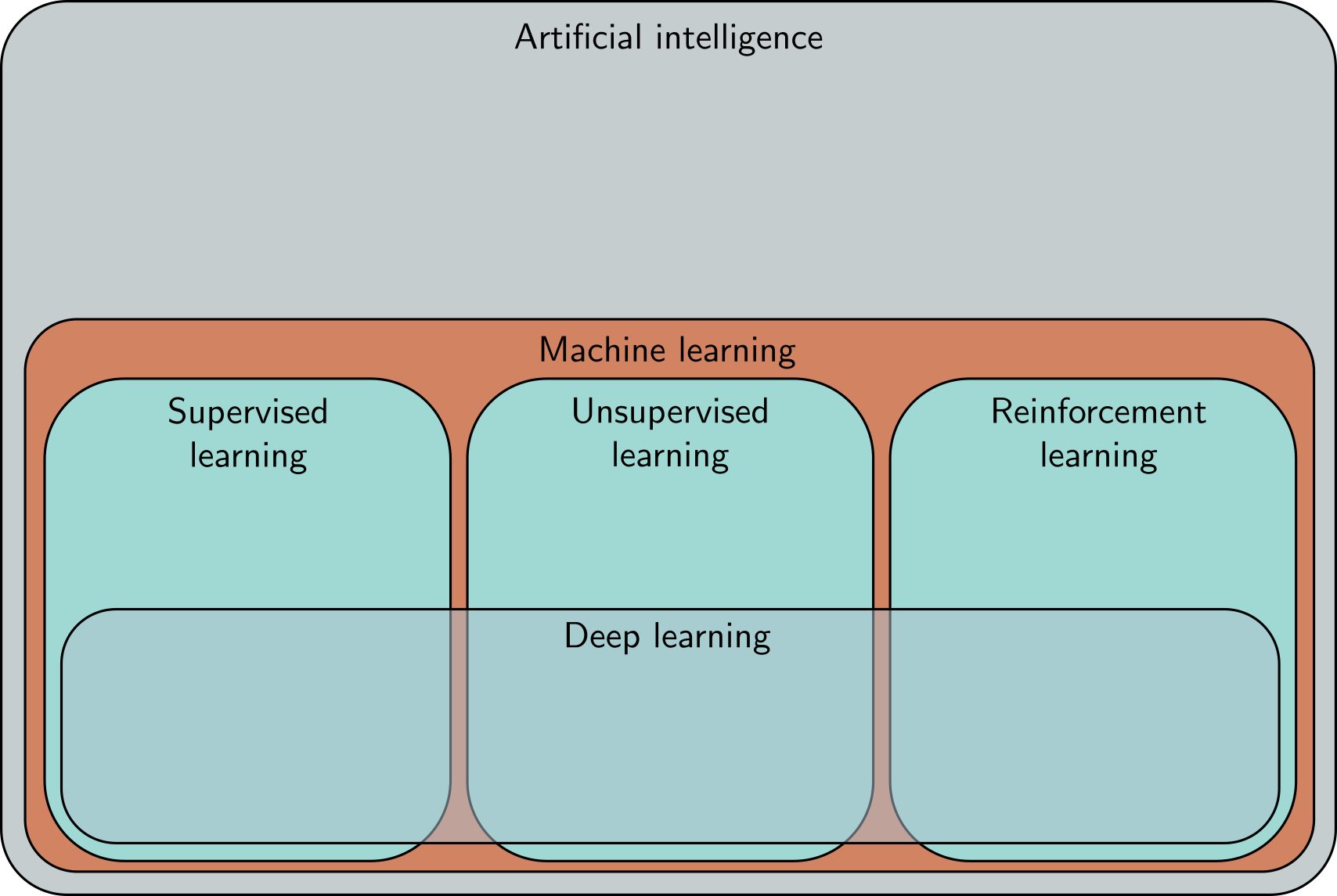
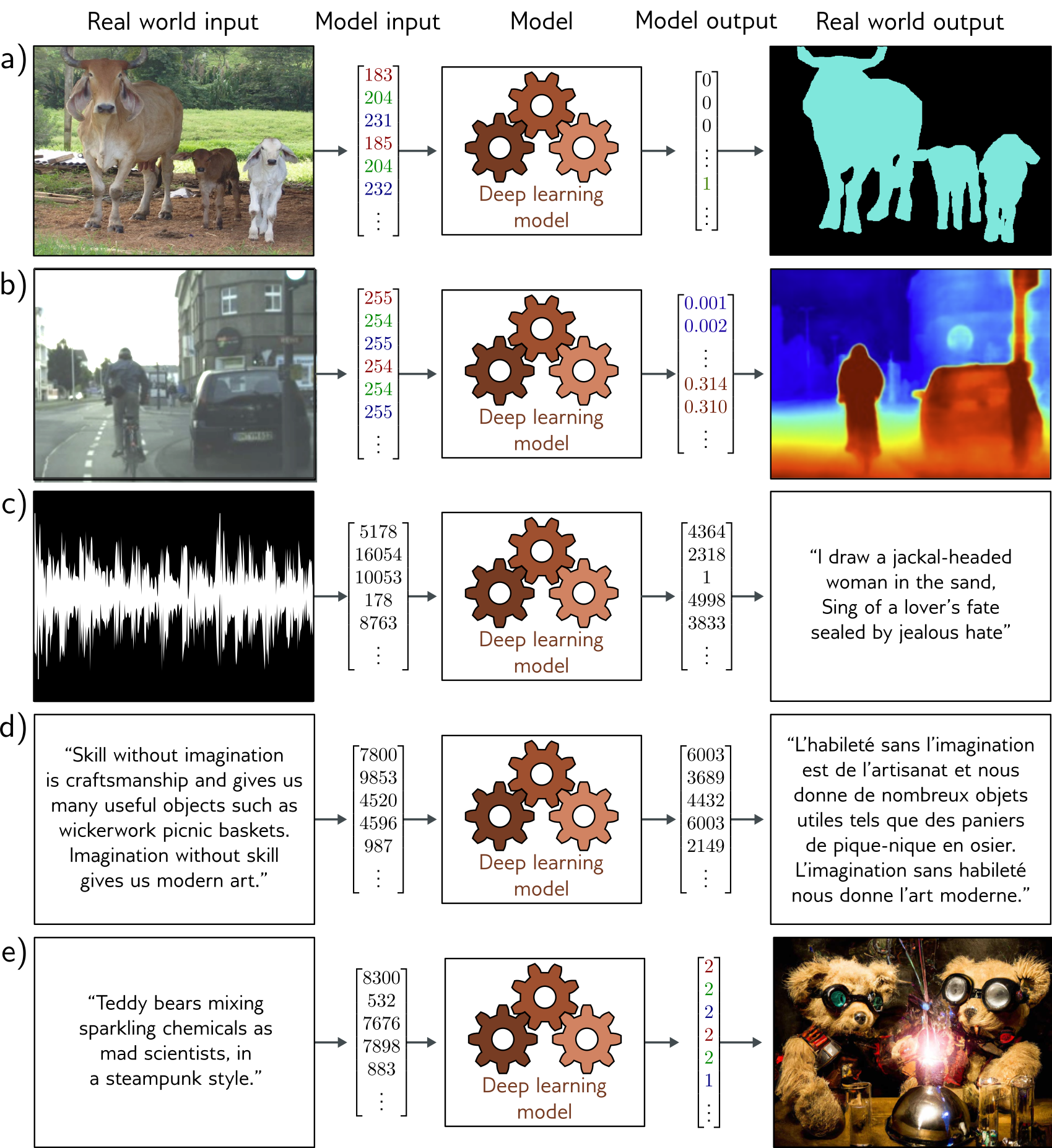
Landscape of AI
Figures from Understanding Deep Learning, by Simon J.D. Prince, used with permission
Supervised Learning
- Given lots of examples of (item, label) pairs
- Learn a function that maps items to labels
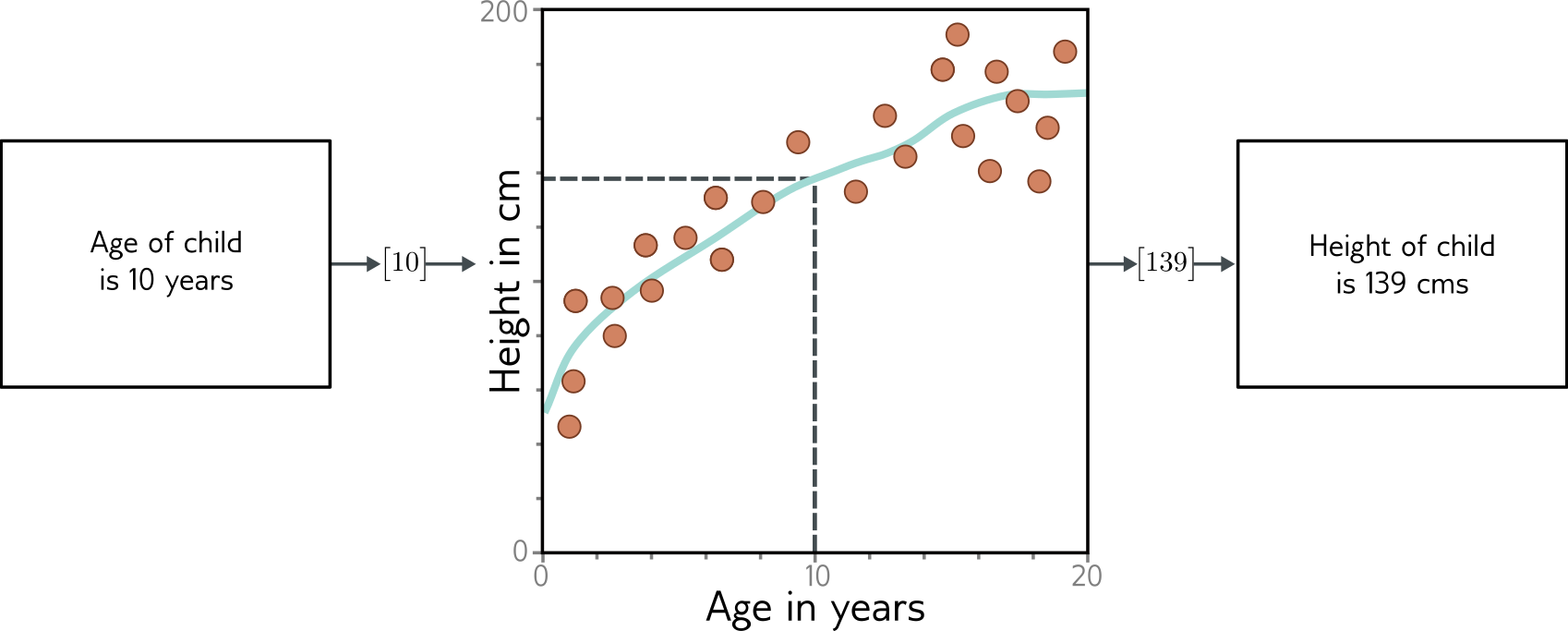
Regression
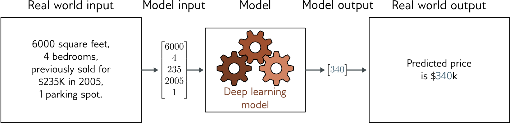
Labels are continuous numbers
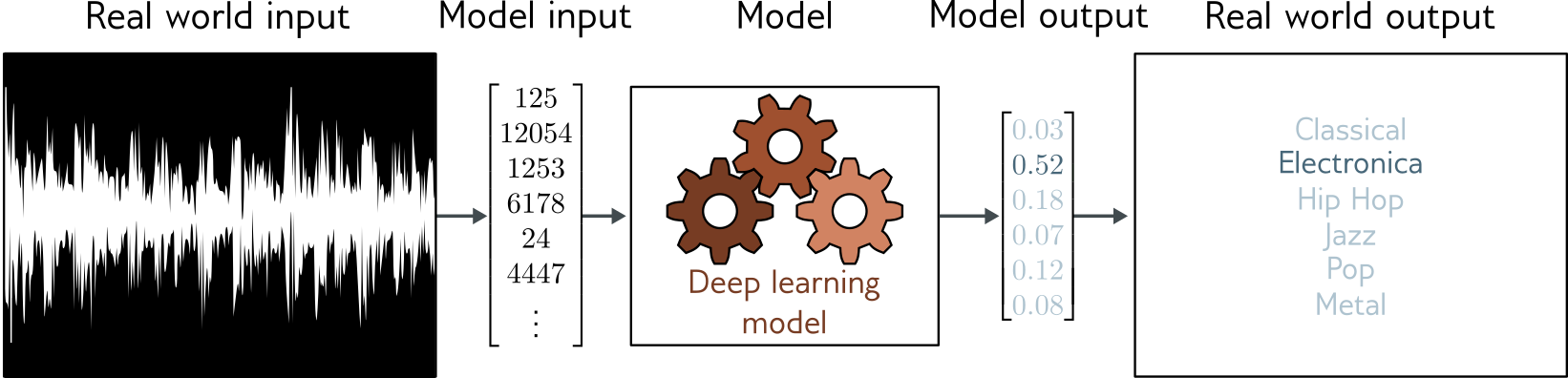
Classification

Labels are discrete categories (so outputs are probabilities)
Supervised Learning Model
- Model is a function from inputs to outputs
- “fitting” the model means searching for a “good” function
- “predicting” means applying the function to new inputs
Types of Labels
Unsupervised Learning
No explicit labels
- Clustering
- Finding outliers
- Filling in missing data
- Generating new data
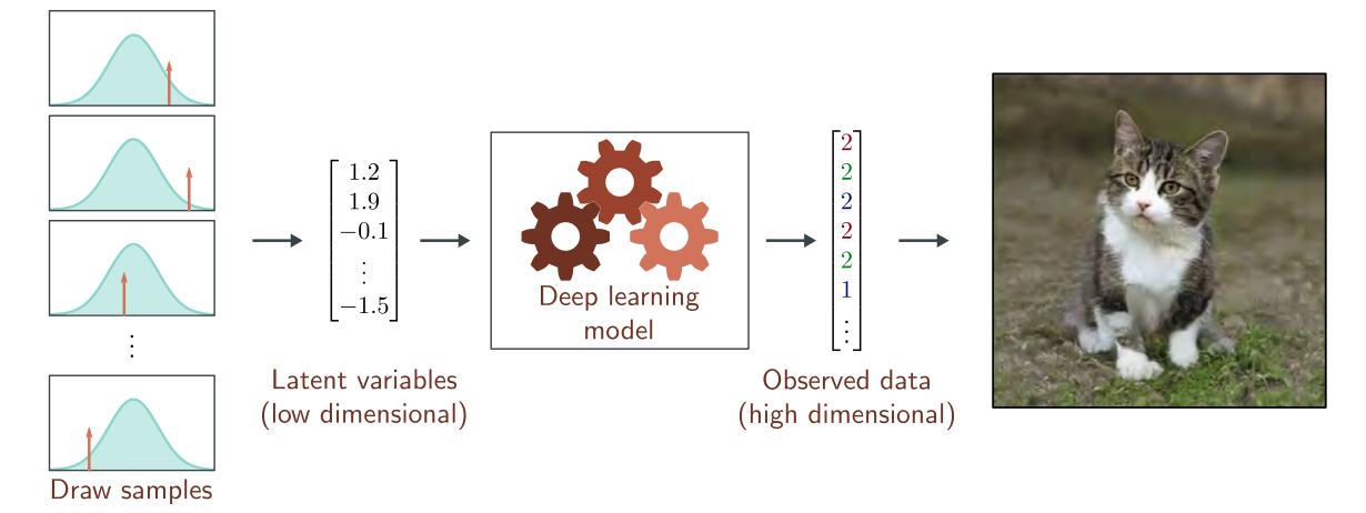
Generative Models
A type of unsupervised learning
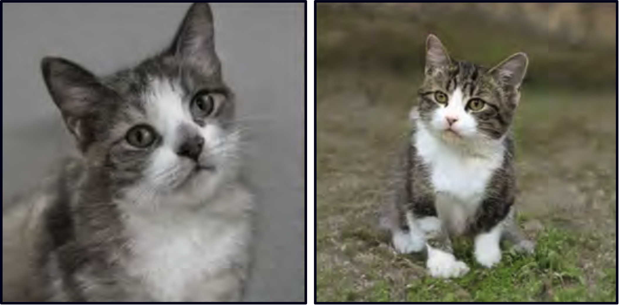
Latent Variables
Conditional Synthesis

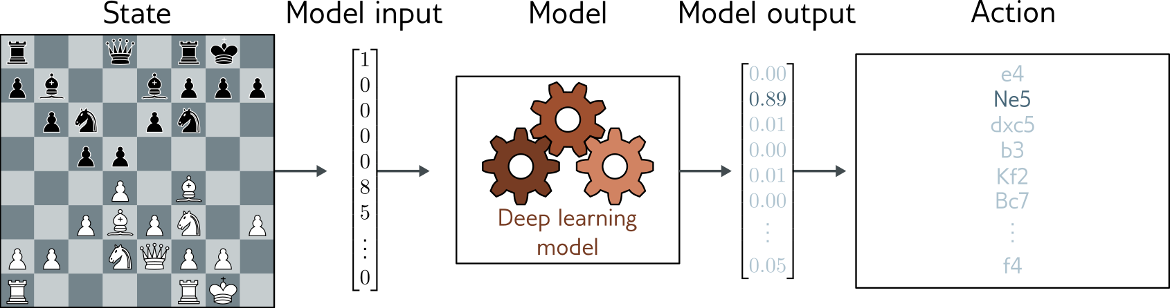
Reinforcement Learning
- Input: perceptions of the world
- Output: actions to take
- Feedback: reward or punishment (potentially delayed)
- Goal: take actions that get the most reward
Example: chess
- Actions: possible moves
- Reward: win or lose
- Challenge: delayed feedback
Why is it hard?
- Credit assignment: which of my moves were good or bad?
- Exploration vs. exploitation: should I stick with what I know or try something new?
- Stochasticity: opponent responds differently each time
Other Examples
- Self-driving cars
- Robotics
- Healthcare (e.g., treatment plans)
- Games (e.g., AlphaGo)
Types of Supervised Learning
Regression vs Classification
- Note: sometimes classes are represented using numbers.
- Would MSE make sense for measuring the error of a classification model?
Debriefing sklearn notebook
Xis the independent variables,ythe dependent. (this terminology is more common in a statistics setting)- in ML, we call the columns of
Xthe features or predictors, andythe target. - The parallel lines of the linear regression are contours of the prediction, which is actually smooth (in fact, too smooth.)
- The descriptions of the plots are not clear. Notice how some of the boundaries are strictly horizontal/vertical while others are not. Notice how some boundaries are sharp while others are not.
- Why might the RF give lines like the tree, but less sharp lines? Answer: it’s the average of a bunch of trees, each of which has those sharp lines, but different ones.
Metrics and Loss Functions
Regression Metrics
- MAE: Mean Absolute Error (“predictions are usually off by xxx units”)
- MSE: Mean Squared Error (“predictions are usually off by xx units^2”)
- RMSE: Root Mean Squared Error (same units as the target)
- MAPE: Mean Absolute Percent Error (“predictions are usually off by yy%”)
- Traditional R^2 (fraction of variance explained)
MAE is like the median (robust to outliers); MSE/RMSE/R2 is like the mean (cares about the magnitude of errors)
All of these are also valid loss functions (i.e., we can use them to train a model).
Classification Metrics
- Accuracy: fraction of correct predictions
- If there’s just two classes (positive and negative), we can also compute:
- Precision: fraction of true positives among all positives
- Recall: fraction of true positives among all actual positives
- (Lots more metrics, especially for multi-class classification, or when we can freely set thresholds)
Partial Credit
- All regression metrics give partial credit for being close
- But not accuracy.
- So it’s hard to learn from mistakes
- Alternative: categorical cross-entropy (log loss)
Intuition: Predicting the outcome of a game
- Suppose you play chess grandmaster Gary Kasparov in chess. Who wins?
- Suppose you play someone with roughly equal skill. Who wins?
Answer as a probability distribution.
Good predictions give meaningful probabilities
- How surprised would you be if you played Gary Kasparov and he won?
- If you won?
- Intuition: surprise
Use surprise to compare two models
Suppose A and B are playing chess. Model M gives them equal odds (50-50), Model Q gives A an 80% win chance.
| Player | Model M win prob | Model Q win prob |
|---|---|---|
| A | 50% | 80% |
| B | 50% | 20% |
Now we let them play 5 games, and A wins each time. (data = AAAAA)
What is P(data given model) for each model?
- Model M:
0.5 * 0.5 * 0.5 * 0.5 * 0.5= (0.5)^5 = 0.03125 - Model Q:
0.8 * 0.8 * 0.8 * 0.8 * 0.8= (0.8)^5 = 0.32768
Which model was better able to predict the outcome?
Likelihood
Likelihood: probability that a model assigns to the data. (The P(AAAAA) we just computed.)
Assumption: data points are independent and order doesn’t matter. (i.i.d). So P(AAAAA) = P(A) * P(A) * P(A) * P(A) * P(A)
Log Likelihood
- Likelihood numbers can quickly get too small to represent accurately.
- Computational trick: take the logarithm.
- log2(.5) = -1 because 2^(-1) = 0.5
- log2((0.5)^5) = 5 * log2(0.5) = 5 * -1 = -5
- log of a product = sum of logs
Log likelihood of data for a model:
- Compute the model’s probability for each data point
- Take the log of each probability
- Sum the logs
Cross-Entropy Loss
- Negative of the log likelihood (“NLL”)
- Intuition: average surprise
- A good regression model predicts nearby the right answer.
- A good classifier should give high probability to correct result.
- Cross-entropy loss = average surprise.
Technical note: MSE loss minimizes cross-entropy if you model the data as Gaussian.
For technical details, see Goodfellow et al., Deep Learning Book chapters 3 (info theory background) and 5 (application to loss functions).
Categorical Cross-Entropy
Cross-entropy when the data is categorical (i.e., a classification problem).
Definition: Average of negative log of probability of the correct class.
- Model M: Gave prob of 0.5 to the correct answer. Cross-entropy loss = -log2(0.5) = 1 bit
- Model Q: Gave prob of 0.8 to the correct answer. Cross-entropy loss = -log2(0.8) = 0.3219 bits
(Usually use natural log, so units are nats.)
Math aside: Cross-Entropy
- A general concept: comparing two distributions.
- Most common use: classification.
- Classifier outputs a probability distribution over classes.
- Categorical cross-entropy is a distance between that distribution and the “true” distribution.
- Estimate the true distribution using a 1-hot vector with 1 in the correct class and 0 elsewhere.
- But it applies to any two distributions.