Computing

Ken Arnold

What is Neural Computing

Key Questions

• How do neural nets compute? (How does that differ from traditional programming?)
• What are the “data structures” of neural computing and efficient operations we can do with them?
• How can we update parameters to optimize an objective function?

Learning Path

“I trained a neural net classifier from scratch.”

1. Basic array/“tensor” operations in PyTorch
   • Code: array operations
   • Concepts: dot product, mean squared error
2. Linear Regression “the hard way” (but black-box optimizer)
   • Code: Representing data as arrays
   • Concepts: loss function, forward pass, optimizer
3. Logistic Regression “the hard way”
   • Concepts: softmax, cross-entropy loss
4. Multi-layer Perceptron
   • Concepts: nonlinearity (ReLU), initialization
5. Gradient Descent
   • Concepts: backpropagation, training loop
6. Data Loaders
   • Concepts: batching, shuffling

Foundations

Lab 1 Review

Open up your Lab 1 notebooks. Discuss with your neighbors:

1. What’s the rule for what outputs you see from a code chunk?
2. What parameter changes did you try in the image classifier? What did you observe?
3. What else did you learn? Is there anything you’d like us to go over together?

Lab Takeaways

• How lab notebooks work
  • self-contained
    • Tasks (marked with “Task”)
    • blank code cells (labeled # your code here)
  • emphasize process over product
  • check-in quizzes on Moodle
• getting set up on Kaggle

Jupyter Notebooks

• notebook = prose + code + output
• interfaces for notebooks: Jupyter (classic and Lab), VS Code, Kaggle, Google Colab (view-only: github, nbviewer)
• cell types
  • Markdown (GitHub Docs, spec)
  • Code
    • Each code block feeds input to a hidden Python repl (“Shell” in Thonny)
      • Possible to run code out of order
      • Changing something doesn’t make dependent code re-run!
    • Outputs: anything explicitly display()ed or print()ed or plot()ted—and the result of the last expression

Model training and Evaluation

• Outline of notebooks
  1. Load the data
     1. Download the dataset.
     2. Set up the dataloaders (which handles train-validation split, batching, and resizing)
  2. Train a model
     1. Get a foundation model (an EfficentNet in our case)
     2. Fine-tune it.
  3. Get the model’s predictions on an image.
• Evaluating a model
  • Accuracy: correct or incorrect?
  • Loss:
    • partial credit
    • when it’s right, should be confident
    • when it’s wrong, shouldn’t be confident

Markdown Tips

aka, things to make your work look more professional

• Headings: space between # and the heading text
• Multiple lines collapse to a single line unless you:
  • Use a list (- abc)
  • Add a blank space between
  • manually add space (advanced technique)
• Use backticks when you’re talking about code (e.g., functions, variable names)

Random Seeds

import random
random.seed(1234)
print(random.random())
print(random.random())

random.seed(1234)
print(random.random())
print(random.random())

1. All four numbers will be different.
2. The first two numbers will be the same, and the second two numbers will be the same.
3. All four numbers will be the same.

import random
random.seed(1234)
print(random.random())
print(random.random())

0.9664535356921388
0.4407325991753527

random.seed(1234)
print(random.random())
print(random.random())

0.9664535356921388
0.4407325991753527

Array Programming: numpy

aka np, because it’s canonically imported as:

import numpy as np

numpy

• Numerical computing library for Python
• Provides the array data type. Like a list but:
  • Automatic for loops!
  • Supports multiple dimensions
• …and lots of utilities
  • arange: range that makes arrays
  • zeros / ones / full: make new arrays
  • lots of math functions

example

x = [1.0, 2.0, 3.0]
y = [3.0, 2.0, 1.0]
x + y

• [4., 4., 4.]
• [1.0, 2.0, 3.0, 3.0, 2.0, 1.0]
• error

import numpy as np
x = np.array([1.0, 2.0, 3.0])
y = np.array([3.0, 2.0, 1.0])
x + y

• [4., 4., 4.]
• [1.0, 2.0, 3.0, 3.0, 2.0, 1.0]
• error

• “broadcasting” = automatic for loops.
• array() representation indicates that it’s an array type.

Arrays have consistent data types

All ints:

np.array([1, 2, 3])

array([1, 2, 3])

All floats:

np.array([1, 2, 3.1])

array([1. , 2. , 3.1])

np.arange

Like range, but:

• makes NumPy arrays
• allows floats

x = np.arange(0.0, 2.0, .5)
x[:5]

array([0. , 0.5, 1. , 1.5])

Broadcasting (automatic for loops!)

array plus scalar:

x + 1

array([1. , 1.5, 2. , 2.5])

array plus array:

x + x

array([0., 1., 2., 3.])

Applying a function to every element:

y = np.sin(2 * np.pi * x)
y

array([ 0.0000000e+00,  1.2246468e-16, -2.4492936e-16,  3.6739404e-16])

Reduction operations

Reduce the dimensionsionality of an array (e.g., summing over an axis)

x.sum()

np.float64(3.0)

x.mean()

np.float64(0.75)

x.max()

np.float64(1.5)

np.argmax(x)

np.int64(3)

Exercise: computing error

Suppose the true values are:

y_true = np.array([1., 2., 3.])

and two model predictions are:

y_pred_a = np.array([1.5, 1.5, 3.5])
y_pred_b = np.array([1.1, 2.1, 1.8])

1. In what sense is Model A better? In what sense is Model B better? Try to quantify the score of each model in at least 2 different ways.
2. Write NumPy expressions to compute each of the errors you listed.

Quantifying Error

Error Metrics

MAE: mean absolute error: average of absolute differences

\[ \text{MAE} = \frac{1}{n} \sum_{i=1}^n |y_i - \hat{y}_i| \]

mae_a = np.abs(y_true - y_pred_a).mean()
mae_b = np.abs(y_true - y_pred_b).mean()

print('MAE a: {:.2f}, MAE b: {:.2f}'.format(
  mae_a, mae_b))

MAE a: 0.50, MAE b: 0.47

MSE: mean squared error or RMSE: root mean squared error

\[ \text{MSE} = \frac{1}{n} \sum_{i=1}^n (y_i - \hat{y}_i)^2 \]

mse_a = ((y_true - y_pred_a) ** 2).mean()
mse_b = ((y_true - y_pred_b) ** 2).mean()

print('MSE a: {:.2f}, MSE b: {:.2f}'.format(
  mse_a, mse_b))

MSE a: 0.25, MSE b: 0.49

Contrasting MAE and MSE

• Which model had a better MAE? Which had a better MSE?
• What do you notice about the specific mistakes that the models made?

pd.DataFrame({
  'y_true': y_true,
  'y_pred_a': y_pred_a, 'err_a': y_true - y_pred_a,
  'y_pred_b': y_pred_b, 'err_b': y_true - y_pred_b,
 }).style.hide(axis='index').format('{:.1f}')

y_true	y_pred_a	err_a	y_pred_b	err_b
1.0	1.5	-0.5	1.1	-0.1
2.0	1.5	0.5	2.1	-0.1
3.0	3.5	-0.5	1.8	1.2

Linear Regression

Model = architecture + loss + data + optimization

From Linear Regression to Neural Networks

CS 375:

• Nonlinear transformations (ReLU, etc.)
• Extend to classification (softmax, cross-entropy loss)
• More layers (“deep learning”)

CS 376:

• Handle structure (locality of pixels in images, etc.)
• Flexible data flow (attention, recurrences, etc.)

Linear Regression with One Output

# inputs:
# - x_train (num_samples, num_features)
# - y_train (num_samples)
num_features_in = x_train.shape[1]
w = np.random.randn(num_features_in)
b = np.random.randn()

y_pred = x_train @ w + b
loss = ((y_train - y_pred) ** 2).mean()

Check-in question: what loss function is this?

Multiple Inputs and Outputs

• y = x1*w1 + x2*w2 + x3*w3 + b
• Or: y = x @ W + b

Matmul (@) so we can process every example of x at once:

• x is 100 samples, each with 3 features (x.shape is (100, 3))
• W gives 4 outputs for each feature (W.shape is (3, 4))
• Then x @ W gives 100 samples, each with 4 outputs ((100, 4))
• Think: what is b’s shape?

Linear Regression with Multiple Outputs

# inputs:
# - x_train (num_samples, num_features_in)
# - y_train (num_samples, num_features_out)
num_features_out = y_train.shape[1]
W = np.random.randn(num_features_in, num_features_out)
b = np.random.randn(num_features_out)

y_pred = x_train @ W + b
loss = ((y_train - y_pred) ** 2).mean()

• W is now a 2-axis array: how much each input contributes to each output
• b is now a 1-axis array: a number to add to each output

Logistic Regression

Code Example

# inputs:
# - x_train (num_samples, num_features)
# - y_train (num_samples, num_classes), one-hot encoded
num_classes = y_train.shape[1]
W = np.random.randn(num_features_in, num_classes)
b = np.random.randn(num_classes)

scores = x_train @ W + b
probs = softmax(scores, axis=1)

probs_of_correct = probs[np.arange(len(y_train)), y_train]
loss = -np.log(probs_of_correct).mean()

Check-in question: what loss function is this?

Intuition: Elo

A measure of relative skill:

• Higher Elo more likely to win
• Greater point spread -> more confidence in win

Formal definition:

Pr(A wins) = 1 / (1 + 10^(-EloDiff / 400))

EloDiff = A Elo - B Elo

• Uses: chess, NFL
• 538’s Superbowl prediction (discussion)
• sometimes adjusted, e.g., for playoffs, 538 multiplies EloDiff by 1.2 (wider margins in playoffs)

From scores to probabilities

Suppose we have 3 chess players:

player	Elo
A	1000
B	2200
C	1010

A and B play. Who wins?

A and C play. Who wins?

Softmax

See nfelo

1. Pick a pair of teams from the list.
2. Compute the difference in their Elo ratings.
3. Compute the probability that the higher-rated team wins.
4. Repeat for another pair of teams.

Elo probability formula:

Pr(A wins) = 1 / (1 + 10^(-EloDiff / 400))

Softmax

1. Start with scores (use variable name logits), which can be any numbers (positive, negative, whatever)
2. Make them only positive by exponentiating:

• xx = exp(logits) (logits.exp() in PyTorch)
• alternatives: 10 ** logits or 2 ** logits

3. Make them sum to 1: probs = xx / xx.sum()

Some properties of softmax

• Sums to 1 (by construction)
• Largest logit in gets biggest prob output
• logits + constant doesn’t change output.
• logits * constant does change output.

Sigmoid

Special case of softmax when you just have one score (binary classification): use logits = [score, 0.0]

Exercise for practice: write this out in math and see if you can get it to simplify to the traditional way that the sigmoid function is written.

Where do the “right” scores come from?

• In linear regression we were given the right scores.
• In classification, we have to learn the scores from data.

Nonlinear Features

ReLU

Chop off the negative part of its input.

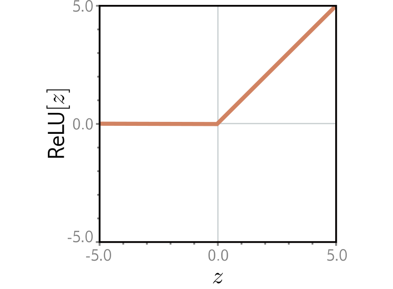
y = max(0, x)

(Gradient is 1 for positive inputs, 0 for negative inputs)

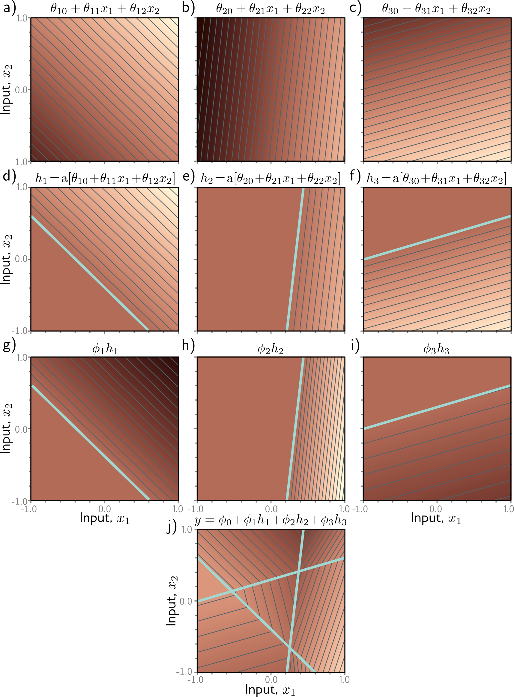
Why is ReLU Useful?

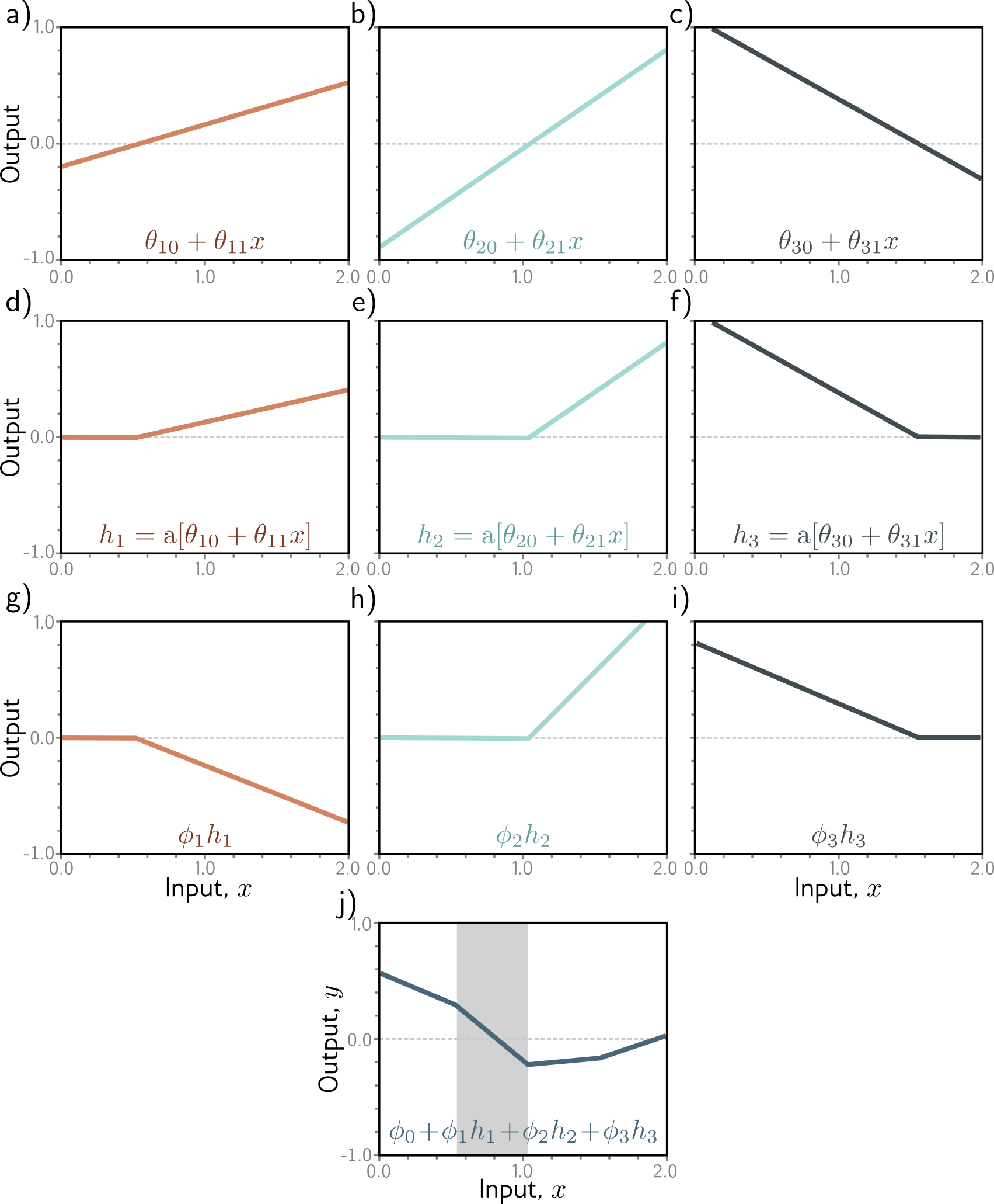
In 2D

Interactive Activity

ReLU interactive (name: u04n00-relu.ipynb; show preview, open in Colab)

Gradient Descent

(Stochastic) Gradient Descent algorithm

1. Get some data
2. Forward pass: compute model’s predictions
3. Loss computation: compare predictions to targets
4. Backward pass: compute gradient of loss with respect to model parameters
5. Update: adjust model parameters in a direction that reduces loss (“optimization”)

• Gradient descent: do this on the whole dataset
• Stochastic Gradient Descent (SGD): do this on subsets (mini-batches) of the dataset

What it looks like in different libraries

PyTorch

import torch
import torch.nn as nn

model = nn.Linear(3, 1)
loss_fn = nn.MSELoss()
optimizer = torch.optim.SGD(model.parameters())
# ...
y_pred = model(x)
loss = loss_fn(y_pred, y)
loss.backward()
optimizer.step()

TensorFlow (low-level)

import tensorflow as tf
import keras

model = keras.layers.Dense(1, input_shape=(3,))
loss_fn = keras.losses.MeanSquaredError()
optimizer = keras.optimizers.SGD()
# ...
with tf.GradientTape() as tape:
    y_pred = model(x)
    loss = loss_fn(y, y_pred)
grads = tape.gradient(loss, model.trainable_weights)
optimizer.apply_gradients(zip(grads, model.trainable_weights))

Automatic Differentiation

• Programmer computes the forward pass
• Library computes the backward pass (gradients) using the backpropagation algorithm
  • Start at the end (loss)
  • Work backwards through the computation graph
  • Use the chain rule to compute gradients

Upshot: we can differentiate programs.

A Story of A Classifier

Images as Input

• Each image is a 3D array of numbers (color channel, height, width) with rich structure: adjacent pixels are related, color channels are related, etc.
• Eventually we’ll handle this, but to simplify for now:
  • Ignore color information: use grayscale images: 28x28 array of numbers from 0 to 255
  • Ignore spatial relationships: flatten to 1D array of 784 numbers

Work through how this is done in the Chapter 2 notebook

Classification the Wrong Way

1. Compute y = x @ W + b to compute a one-dimensional output y for each image.
2. Compute the MSE loss between y and the desired number (0-9).
3. Optimize the weights to minimize this loss.

Discuss with neighbors:

1. Suppose you’re trying to classify an image of a 4. What might a prediction from this model look like? Compute the loss.
2. What’s wrong with this approach? What might you do instead?

Fix 1: Multiple Outputs

We want a score for each digit (0-9), so we need 10 outputs.

Each output is 0 or 1 (“one-hot encoding”).

Discuss with neighbors:

1. What’s the shape of the output?
2. What must be the shape of the weights?
3. What might an output from this model look like when given an image of a 4? What’s the loss?

Fix 2: Softmax (Large Values)

Suppose the network predicted 1.5 for the correct output.

Suppose instead the network predicted 0.5 for the correct output.

What’s the loss in each case?

Fix: make outputs be probabilities.

1. Exponentiate each output
2. Divide by the sum of all exponentiated outputs

Discuss with neighbors:

1. What might an output from this model look like? What’s the loss for your running example?

Fix 3: Cross-Entropy Loss

Negative log of the probability of the correct class.

Compute the loss for your running example.

Embeddings

The internal data structure of neural networks.

General Neural Network Architecture

• Initial layers extract features from input
• Final layers make decisions based on those features

flowchart LR
    A[Input] --> B[Feature Extractor]
    B --> C[Linear Classifier]
    C --> D[Output]

Example:

flowchart LR
    A[Input] --> B["Pre-trained CNN"]
    B --> C["Linear layer with 3 outputs"]
    C --> D["Softmax"]
    D --> E["Predicted probabilities"]
    style B stroke-width:4px

Your Homework 1 Architecture

• The Feature Extractor is composed of:
  • a convolutional neural network …
  • pre-trained on some classification task …
  • with the linear classifier removed
• Linear Classifier: a linear layer plus a softmax (like we’ve been using)

The feature extractor constructs a representation of the input that’s useful for classification.

• A linear classifier on the raw pixels couldn’t learn much.
• A linear classifier on the features extracted by a CNN can learn a lot.
• The CNN computes an embedding of the input image.

The Data Structures of Neural Computing

• Array / Tensor: the basic data structure
• We’ve used them in a few different ways
  • Inputs to the model
    • sometimes each entry is meaningful (e.g., characteristics of a home, vitals of a patient)
    • sometimes entries only meaningful in aggregate (e.g., pixels in an image)
  • Outputs of the model (predictions, targets)
  • Parameters of the model (weights, biases)
  • Intermediate computations (e.g., logits, gradients)
  • Embedding: what we’ll talk about today

Defining Embeddings

Embedding noun: a vector representation of an object, constructed to be useful for some task (not necessarily human-interpretable); verb: to construct such a representation.

Similar items get similar embeddings.

Similarity can be defined as:

• Euclidean distance
• Dot product
• Cosine similarity

(Note: some sources describe “embedding” as a specific lookup operation, but we’ll use it more broadly.)

Example: Word Embeddings

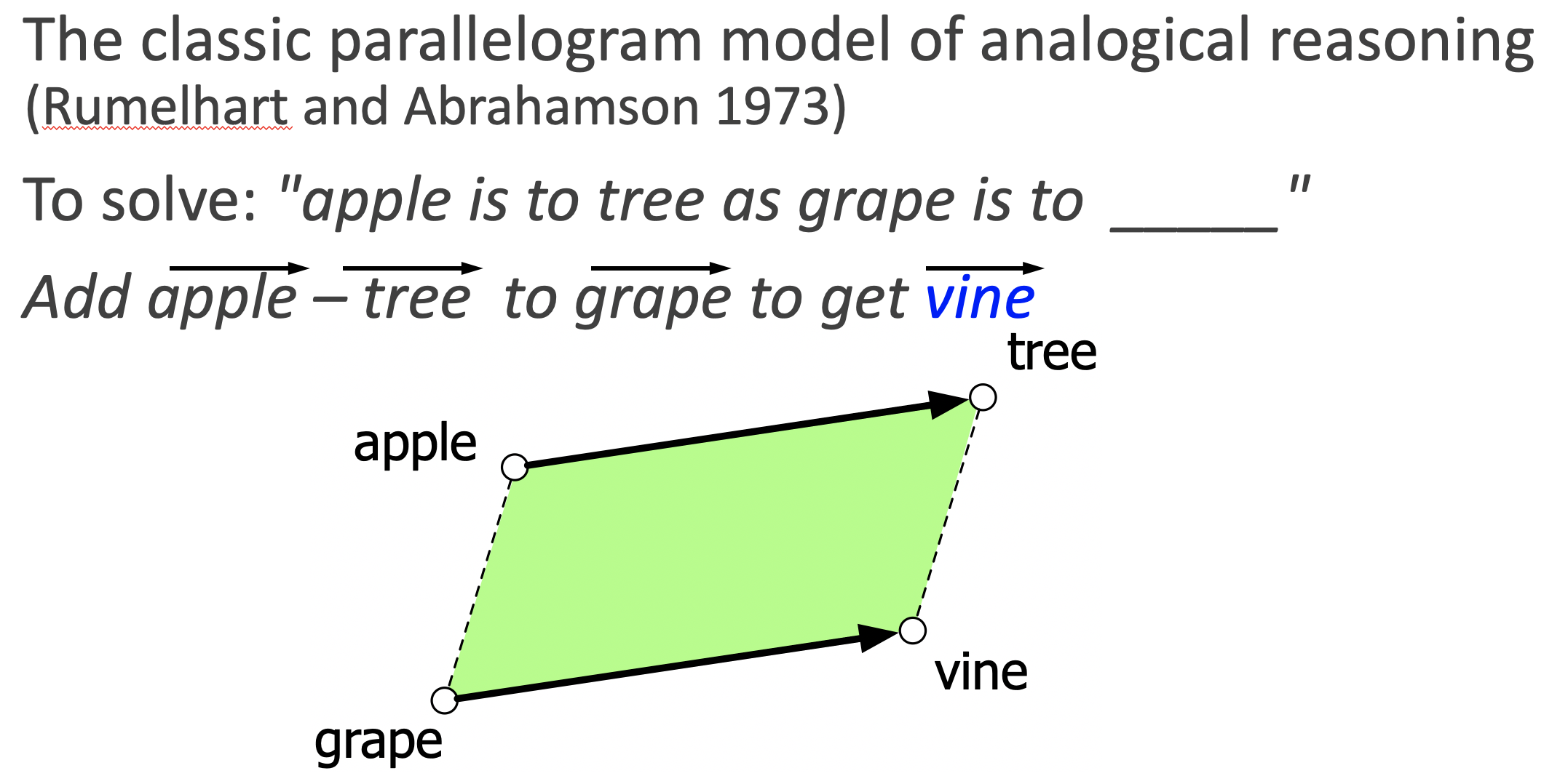
Source: Jurafsky and Martin. Speech and Language Processing 3rd ed

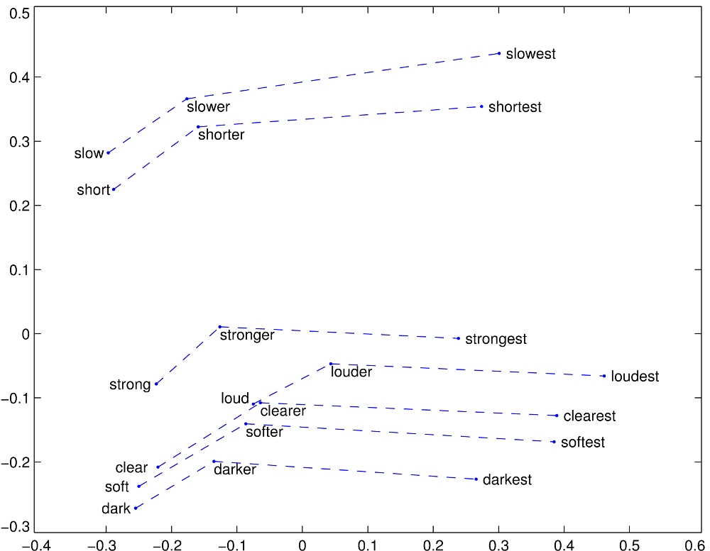
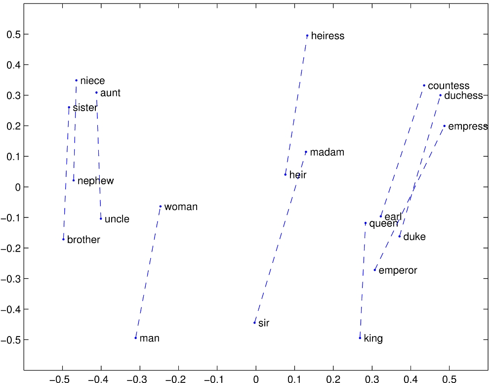
See also: Word embeddings quantify 100 years of gender and ethnic stereotypes (Garg et al, PNAS 2018)

Source: GloVe project

Example: Movie Recommendations

• Each movie gets an embedding vector (analogy: genres)
• Each user gets an embedding vector (analogy: genre preferences)
• Predict rating as dot product of user and movie vectors

Similar people end up with similar vectors because they like similar movies.