HPC MPI Exercise 4: Hands-On Lab, Part 2

Part 2: Collective Communication and Parallel I/O

In part 1 of this week's exercise, we explored different ways to improve the performance of sequential I/O.

A. Collective Commmunication

In this second part of this week's exercise, we'll start by exploring MPI's Collective Communications patterns, which include:

1. The broadcast pattern.
2. The reduction pattern.
3. The scatter pattern.
4. The gather pattern.
5. The the scatterv and gatherv patterns.

In your folder for this week's work, for each pattern: create a new folder and download the source program and Makefile to that folder. Build and run the program, and compare its output to the source. Use the exercise described in the source program's opening comment to experiment with the program, until you understand how the pattern works.

When you are comfortable with each of these communication patterns and understand how they differ from one another, continue on to Section B.

B. HPC I/O Before MPI-2

The remainder of this week's lab exercise is to continue to explore different aspects of file input, but for parallel (MPI) programs instead of sequential programs. As in part 1, we will all read from the same set of (large) data files, which are stored in the directory: /home/cs/374/exercises/04/.

Prior to the release of the MPI-2 standard, there was no portable, free, open-source parallel I/O mechanism. Instead, if a program needed to read data from an input file, the convention was to use the Master-Only and Scatter patterns, as follows:

1. The Master reads the data from the input file into an array.
2. Scatter the Master's array to all the PEs.

• Waste memory by allocating a bigger-than-necessary array whose size is evenly divisible by P (so that we can use MPI_Scatter()); or
• Use the MPI_Scatterv() function, which requires a fair amount of work to set up.

If necessary, use cd to change to your directory for this exercise. There, make a new directory named readScatter, cd to that directory, and then download the files readScatter.c, chunks.h, and Makefile from this folder to that directory.

Using a text editor, open the file readScatter.c and take a few minutes to study its contents.

Discuss with your neighbor: After the Master process reads the values from the file into the array, what steps are needed to scatter that array to all PEs?

To save you time, we have already added MPI_Wtime() timing calls and modified the final printf() so that the program computes and reports the times required to (i) read the file into the array, (ii) scatter the array, and (iii) perform the full computation.

Using the provided Makefile, build the readScatter program; then use your genHosts.pl script to create a hosts file. The readScatter program uses the fread() command, which requires the input file to be in the binary format, so run readScatter, using the command:

   mpirun -np 1 -machinefile hosts ./readScatter /home/cs/374/exercises/04/1m-doubles.bin

In the spreadsheet you used for Part 1 of this exercise, add a new row Read+Scatter. Beneath it, add a row of column headings: P, N, Trial 1 Read, Trial 1 Scatter, Trial 1 Total, Trial 2 Read, Trial 2 Scatter, Trial 2 Total, Trial 3 Read, Trial 3 Scatter, Trial 3 Total, Minimum Read, Minimum Scatter, Minimum Total, Speedup, and Efficiency. In the next row, add 1 below P, 1000000 below N, and the times reported by readScatter below the Trial 1 columns. Run the program twice more and add the times below the Trial 2 and Trial 3 columns. Then below the Minimum columns, use a spreadsheet function to compute the minimum read, scatter, and total times for the three trials.

Repeat these steps for the same value of P (1) but different values of N using the files /home/cs/374/exercises/04/10m-doubles.bin, /home/cs/374/exercises/04/100m-doubles.bin, and /home/cs/374/exercises/04/1b-doubles.bin. If the 1b-doubles.bin file takes more than a minute, just use a single trial for it.

Then repeat these steps for the four files using P = 2, 4, 6, and 8.

Make a quick line-chart with Total Time on the vertical axis and P = 1, 2, 4, 6, and 8 on the horizontal axis. Then add data-series for your N = 1M, 10M, 100M, and 1B total time values.

Discuss with your neighbor: What happens to the time as P increases? Is readScatter behaving as you would expect? Why or why not? Which is contributing more to the total time, reading the data from the file or scattering it? What are the implications of this for parallel speedup and efficiency?

Next, use a spreadsheet formula to compute the appropriate values in the Speedup and Efficiency columns for P = 2, 4, 6, and 8. Under the Speedup column, compute the parallel speedup using the formula:

   SpeedupP(N) = Time1(N) / TimeP(N)

Under the Efficiency column, compute the parallel efficiency using the formula:

   EfficiencyP(N) = SpeedupP(N) / P

Discuss with your neighbor: Recall that when using P PEs to solve a problem, the ideal Speedup is P and the ideal Efficiency is 100%, what can we say about the Speedup and Efficiency using the read-and-scatter approach? What happens to each as P increases?

Optional Activity. To gauge the effects of the network on our results, repeat the activities of this Section (B), but run the program without using the -machinefile hosts switch. (Recall that when you do this, mpirun will launch all the processes on your local workstation, so all communication [e.g., broadcast, scatter] will take place within your machine instead of across the network.) How do these results compare to those produced when using -machinefile hosts?

C. Parallel Binary Input

The MPI-2 standard included MPI-IO, a portable, platform-independent mechanism for performing input and output in parallel.

For input, the basic approach is to have each MPI process complete the following steps::

1. Open the file (using a special MPI collective operation).
2. Compute the size of the file.
3. Use the size of the file and the number of MPI processes to logically divide the file into P contiguous chunks that are as equal in size as possible.
4. Use its MPI rank to determine the size of its chunk and the offset of that chunk within the file.
5. Allocate an array big enough to hold its chunk and read its chunk from the file into that array.
6. Close the file (another special MPI collective operation).

Use cd .. to change to the parent directory, make a new directory there named parallelBinIn, cd to that directory, and then download the files parRead.cpp, OO_MPI_IO.h, and Makefile from this folder to that directory.

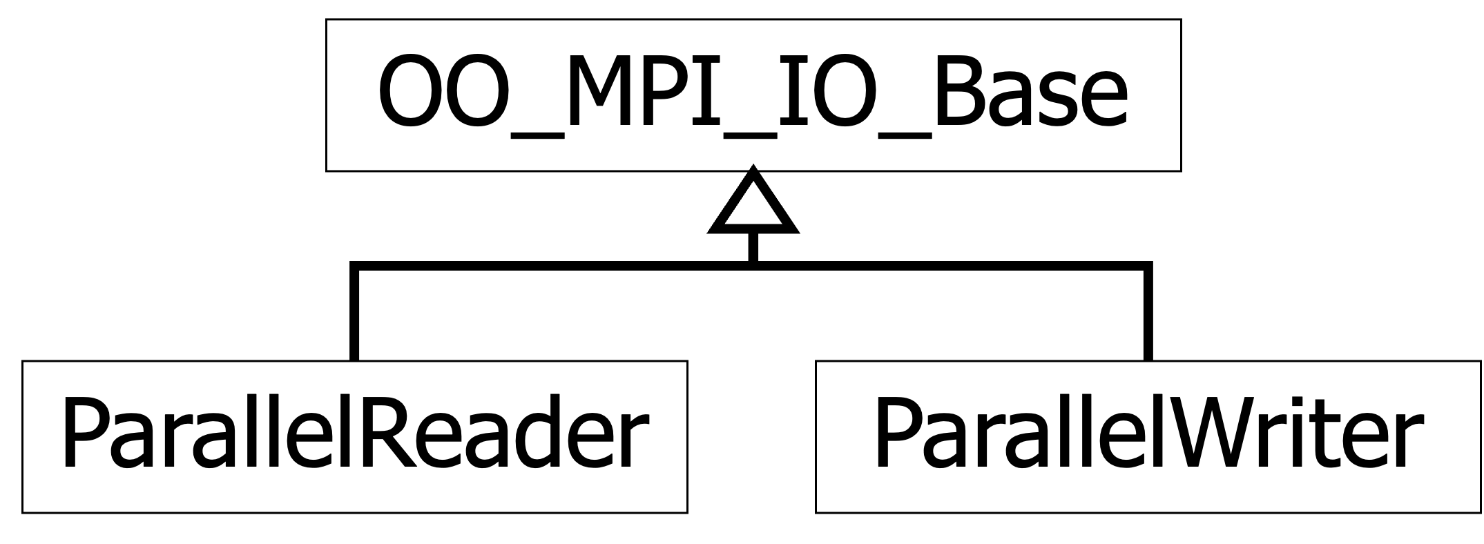
Note that these are C++ files, not C, so the Makefile specifies mpic++ for its compiler and other C++ settings. As you might guess from the name of the file OO_MPI_IO.h, it uses object-oriented thinking to create abstractions that use MPI-IO to perform parallal I/O but hide its complexity. More precisely, OO-MPI-IO.h declares three class templates, which are:

1. ParallelReader, a class template whose constructor and readChunk() methods simplify using MPI-IO's capabilities to let MPI processes read from a binary file in parallel.
2. ParallelWriter, a class template whose constructor and writeChunk() methods simplify using MPI-IO's capabilities to let MPI processes write to a binary file in parallel.
3. OO-MPI-Base, a superclass template of ParallelReader and ParallelWriter that consolidates the functionality they have in common.

We will be using ParallelReader in this last part of today's exercise.

As before, examine parRead.cpp and take a few minutes to compare its contents to the files we have used previously. Things to note include:

• The statements that open the file, read the binary values, and close the file are now implementation details hidden within the ParallelReader abstraction.
• We pass the C/C++ type of value being read from the file (i.e., double in this case) as an argument to the template.
• We pass the equivalent MPI type of the value being read (e.g., MPI_DOUBLE) as an argument to the ParallelReader constructor.
• The ParallelReader abstraction provides a readChunk() method that takes a C++ vector as its argument, and fills that vector with this MPI process's chunk of the input file. All the details of determining the size of the file, the size of this process's chunk, this process's offset within the file, the resizing of the vector, and so on, are hidden within that method.
• To save you time, we have already added the calls to MPI_Wtime() and modified the final printf() so that the program computes and reports the time required to read this process's chunk of the file and the total time.

Use make to build the program; when it builds correctly, use the genHosts.pl to generate a fresh hosts file. Then run the program by entering:

   mpirun -np 1 -machinefile hosts ./parRead /home/cs/374/exercises/04/1m-doubles.bin

[Optional: If you wish to quickly check that this is working correctly, one way is to go to a point after the MASTER-only at the end and add a new printf() statement that displays the size of each MPI process's vector. Since readChunk() is returning a process's chunk of the file in that vector, its size should be equal to that process's chunk-size. For example, using one million values, each process's vector-size should be 500000 when P = 2 and 250000 when P = 4. When P = 3, process 0's vector-size should be 333334 but process 1 and 2's vector-sizes should each be 333333.]

In your spreadsheet, make a new section named Parallel Binary Input, P = 1, with column headings underneath that similar to the preceding section. Run your program two more times, enter the three times under the appropriate Trial columns, and compute the minimum of those trials in the Minimum column.

Then make a new section named Parallel Binary Input, P = 2, with similar column headings plus Speedup and Efficiency column headings.

Run your program three times again using P = 2 and record its times beneath the appropriate columns. Under the Speedup and Efficiency columns, compute the parallel speedup and efficiency for P = 2 and N = 1,000,000.

Then repeat this procedure for P = 2 using the other binary files 10m-doubles.bin, 100m-doubles.bin, and 1b-doubles.bin.

Repeat this full procedure using P = 4, 6, and 8 processes. Consult your neighbor if you have questions.

Wrap up this exercise by creating three quick line-charts to visualize the data you have collected for Parallel Binary Input:

1. A chart showing how the Input Time (Y-axis) changes as the number of processes (X-axis) change, for P = 1, 2, 4, 6, 8.
2. A chart showing how the Speedup (Y-axis) changes as the number of processes (X-axis) change, for P = 2, 4, 6, 8.
3. A chart showing how the Efficiency (Y-axis) changes as the number of processes (X-axis) change, for P = 2, 4, 6, 8.

Congratulations -- You are ready to proceed to this week's project!

Optional:

• Local vs. Remote Files. As noted at the beginning of Part II, the input files we have read are stored on a network file server. Storing files on a network file server provides convenient access from any lab workstation, but it can add significantly to the time required to access a file, compared to files stored locally on a workstation. Each of the CS lab workstations has a local solid state device (SSD) and any files stored in the directory /scratch are stored on this SSD. If you wish to compare the access times for files stored on the network file server vs. files stored on a local SSD, feel free to make a 374 folder in /scratch, copy the files from /home/cs/374/exercises/04 to /scratch/374, and then rerun the programs from this exercise using those local files as the input files to your programs (e.g., /scratch/374/1m-doubles.bin). Note that since /scratch is local to each workstation, you will lose the convenience of being able to work from any workstation in the lab -- you will only be able to access those files from that workstation.
• Input vs. Output Files. In this exercise, we have focused on input. If you are interested in exploring output, the folder parWrite provides the output equivalent of parRead.

CS > 374 > Exercise > 04 > Hands-On Lab