Objectives

Students who complete this lab will demonstrate that they can:

User-Defined Methods

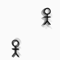
Methods allow programs to add new procedural abstractions to the programming language. In this lab exercise, for example, you write a method to draw a composite stick figure.

Exercise 4b.1:

Create a program called StickFigure that renders the (non-animated) stick figure shown to the right. There are a number of approaches to doing this; for the sake of this exercise, use the following algorithm, which includes a user-defined method :

  • Setup:
    1. Set the output panel size;
    2. Turn on smoothing;
    3. Turn off animation looping.
  • Draw:
    1. Call the method that renders the stick figure.
  • Render figure:
    1. Create a method called renderFigure that receives no arguments.
    2. Set local float variables x and y to the center of the output window;
    3. Set local variable diameter (the diameter of the figure’s head) to 24;
    4. Draw the figure’s trunk;
    5. Draw the figure’s arms;
    6. Draw the figure’s two legs;
    7. Draw the figure’s head.
    This routine returns nothing (i.e., void ) to its calling program.

We suggest that you center the figure’s head at coordinates ( x , y ) and draw all the rest of figure relative to these coordinates. For example, the trunk is a single vertical line from ( x , y + diameter * 0.5 ) to ( x , y + diameter * 1.5 ). This scaling will help you in the next exercise.

Save this program so you can turn it in later.

One nice feature of the code in the previous exercise is that it groups all the figure-drawing code in one appropriately named method. This improves the readability of the program and encourages reuse of that method.

Exercise 4b.2:

Save a copy of your previous program as Parameterized . Modify this new copy so that you can draw two stick figures at different locations (as shown on the right). You can do this as follows:

  • Modify renderFigure() method so that it receives its x and y coordinates from its calling program rather than declaring them locally.
  • Modify draw() so that it invokes renderFigure() twice, passing different x-y coordinates as arguments to each call (e.g. renderFigure(50, 50));

Save this program; you’ll use it as the basis for both exercise 3 and exercise 4.

Methods are valuable for building useful procedural abstractions. We don't need to restrict ourselves to parameterizing just the x-y coordinates of the stick figure.

Exercise 4b.3:

Save a copy of your parameterized program from exercise 2 as Animated . Modify your program to animate a growing (or shrinking) stick figure. The example on the right shows two stationary figures, each growing at different rates. Implement this as follows:

  • Add global variables to represent the diameters of your two stick figures;
  • Add a third parameter to renderFigure() that specifies the diameter of the stick figure and modify the method to draw a scalable stick figure based on this new parameter.
  • Modify draw() to pass the new diameter values as arguments to renderFigure() and to increment the diameter values on each frame.

Save this version of your program so that you can turn it in later.

Methods can also return values. This is useful when your program must compute a certain value frequently.

Exercise 4b.4:

Save a (second) copy of your parameterized program from exercise 2 (not the scalable program from exercise 3) as Brownian . In this exercise, you will modify this program so that it animates the two stick figures using Brownian motion (as shown on the right).

Start by implementing a utility method that helps you constrain the location of your figures, keeping them on the visible canvas at all times. You had to perform a similar task for the Brownian motion exercise in lab 4a. Use the following algorithm:

  • computeCoordinate():
    1. Receive from the calling program: a coordinate value value, a minimum legal value lowerBound and a maximum legal value upperBound;
    2. Compute and return a new value that is randomly modified from value but constrained by lowerBound and upperBound. As in lab 4a, use the constrain method method for this computation.

This method receives a coordinate, either x or y, and returns a new, legal value based on its lower and upper bound arguments. For example, if currentX and currentDiameter refer to the value of a stick figure’s current x coordinate and diameter respectively, then invoking:

computeCoordinate(currentX, currentDiameter/2, 
                 WIDTH - currentDiameter/2)
will return a new value that ensures that the stick figure is not too far to the left or to the right. Test this method by printing out its value for a few key test cases, e.g.: values that are in the range, too small for the range, too large for the range and on the boundaries.

With this utility method in place, you can implement two stick figures this as follows:

  • Add global variables x1, y1, x2 and y2 to store the current coordinates of each of your two stick figures;
  • Modify draw() so that it changes the values of the new global variables by some small amount (e.g., 5 pixels), using your new computeCoordinate() to help you change and constrain the coordinate values;

Save this program so that you can turn it in later.

Exercise 4b.5: Extra Credit

Modify your program so that the color of the stick figure is based on how far it is from some location (or figure). For example, the image to the right shows two animated stick figures that get redder the closer they get to the sun. To do this, you’ll need to use a distance method such as Processing’s dist() method.

Checking In

Submit all the code and supporting files for the exercises in this lab. We will grade this exercise according to the following criteria: